Welcome to the second installation of the Spark and Scylla series. As you might recall, this series will revolve around the integration of Spark and Scylla, covering the architectures of the two products, strategies to transfer data between them, optimizations, and operational best practices.

Last time, we surveyed Spark’s RDD abstraction and the DataStax Spark connector. In this post, we will delve more deeply into the way data transformations are executed by Spark, and then move on to the higher-level SQL and DataFrame interfaces provided by Spark.

The code samples repository contains a folder with a docker-compose.yaml for this post. So go ahead and start all the services:

docker-compose up -d

The repository also contains a CQL file that’ll create a table in Scylla that we will use later in the post. You can execute it using:

docker-compose exec scylladb-node1 cqlsh -f /stocks.cql

Once that is done, launch the Spark shell as we’ve done in the previous post:

Spark’s Execution Model

Let’s find out more about how Spark executes our transformations. As you recall, we’ve introduced the RDD – the resilient, distributed dataset – in the previous post. An instance of RDD[T] is an immutable collection of elements of type T, distributed across several Spark workers. We can apply different transformations to RDDs to produce new RDDs.

For example, here’s an RDD of Person elements from which the ages are extracted and filtered:

If you paste that snippet into the REPL, you’ll note that the runtime type of ages is a MapPartitionsRDD. Here’s a slightly simplified definition of it:

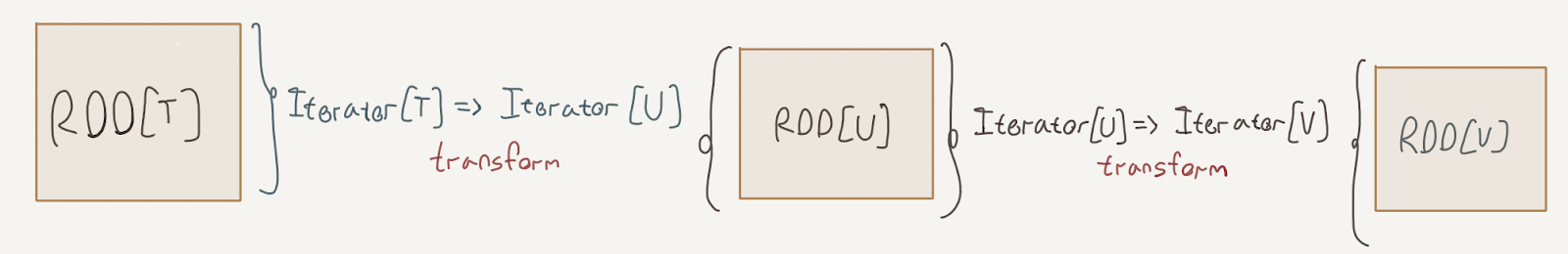
Every transformation that we apply to an RDD – be it map, filter, join and so forth – results in a specialized subtype of RDD. Every one of those subtypes carries a reference to the previous RDD, and a function from an Iterator[T] to an Iterator[U].

The DAG that we described in the previous post is in fact reified in this definition; the previous reference is the edge in the graph, and the transform function is the vertex. This function, practically, is how we transform a partition from the previous RDD to one on the current RDD.

Now, let’s launch the Spark application UI; it is available at http://localhost:4040/. This interface is essential to inspecting what our Spark application is doing, and we’ll get to know some of its important features now.

This is how things are looking after pasting the previous snippet into the REPL:

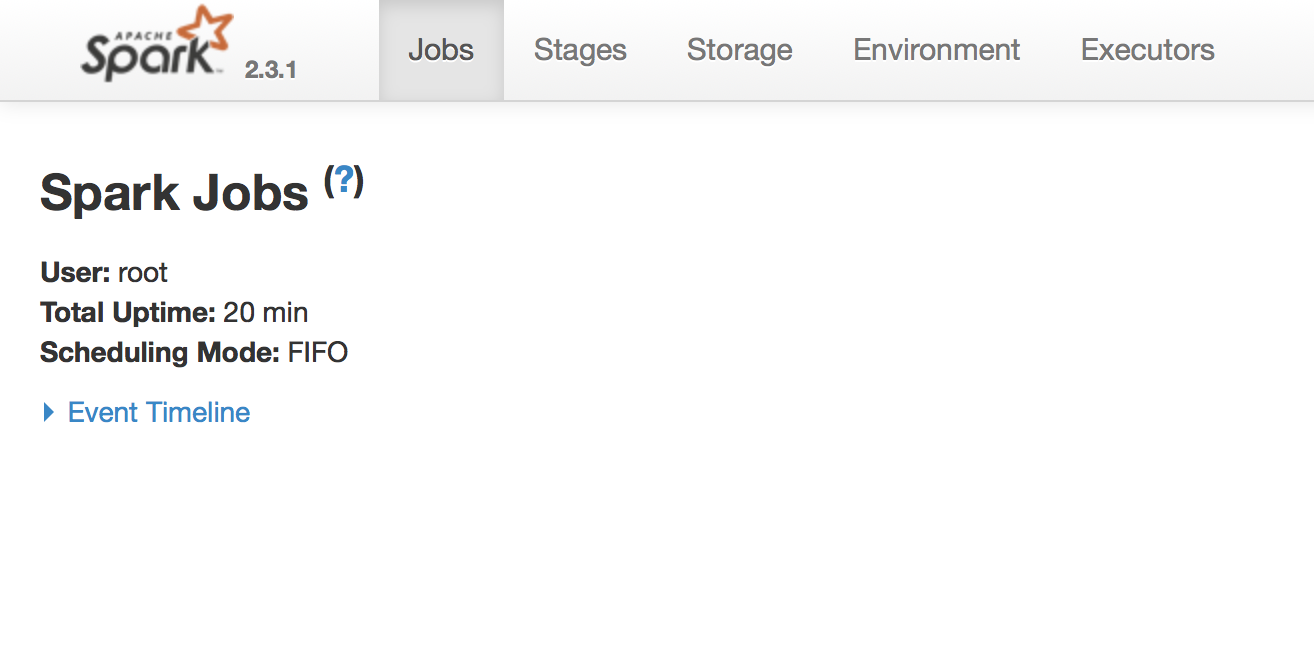
Rather empty. This is because nothing’s currently running, and nothing, in fact, has run so far. I remind you that Spark’s RDD interface is lazy: nothing runs until we run an action such as reduce, count, etc. So let’s run an action!

ages.count

After the count executes, we can refresh the application UI and see an entry in the Completed Jobs table:

This would be a good time to say that in Spark, a job corresponds to an execution of a data transformation – or, a full evaluation of the DAG corresponding to an RDD. A job ends with values outside of the RDD abstraction; in our case, a Long representing the count of the RDD.

Clicking on the description of the job, we can see a view with more details on the execution:

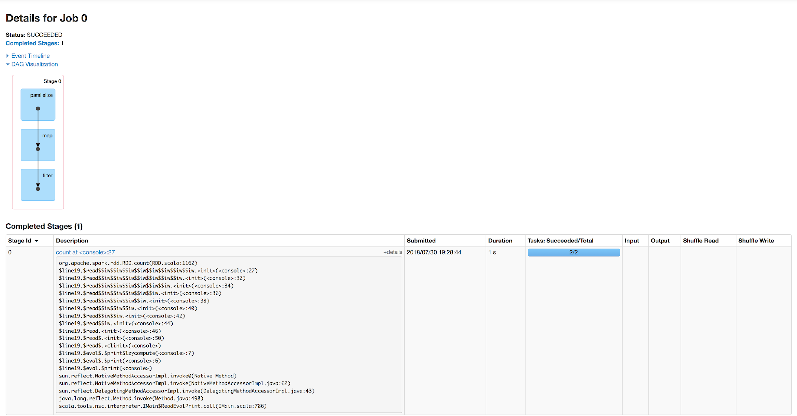
The DAG visualization shows what stages the job consisted of, and the table contains more details on the stages. If you click the +details label, you can see a stack trace of the action that caused the job to execute. The weird names are due to the Scala REPL, but rest assured you’d get meaningful details in an actual application.

We’re not ready yet to define what exactly a stage is, but let’s drill down into the DAG visualization. Clicking on it, we can see a view with more details on the stage:

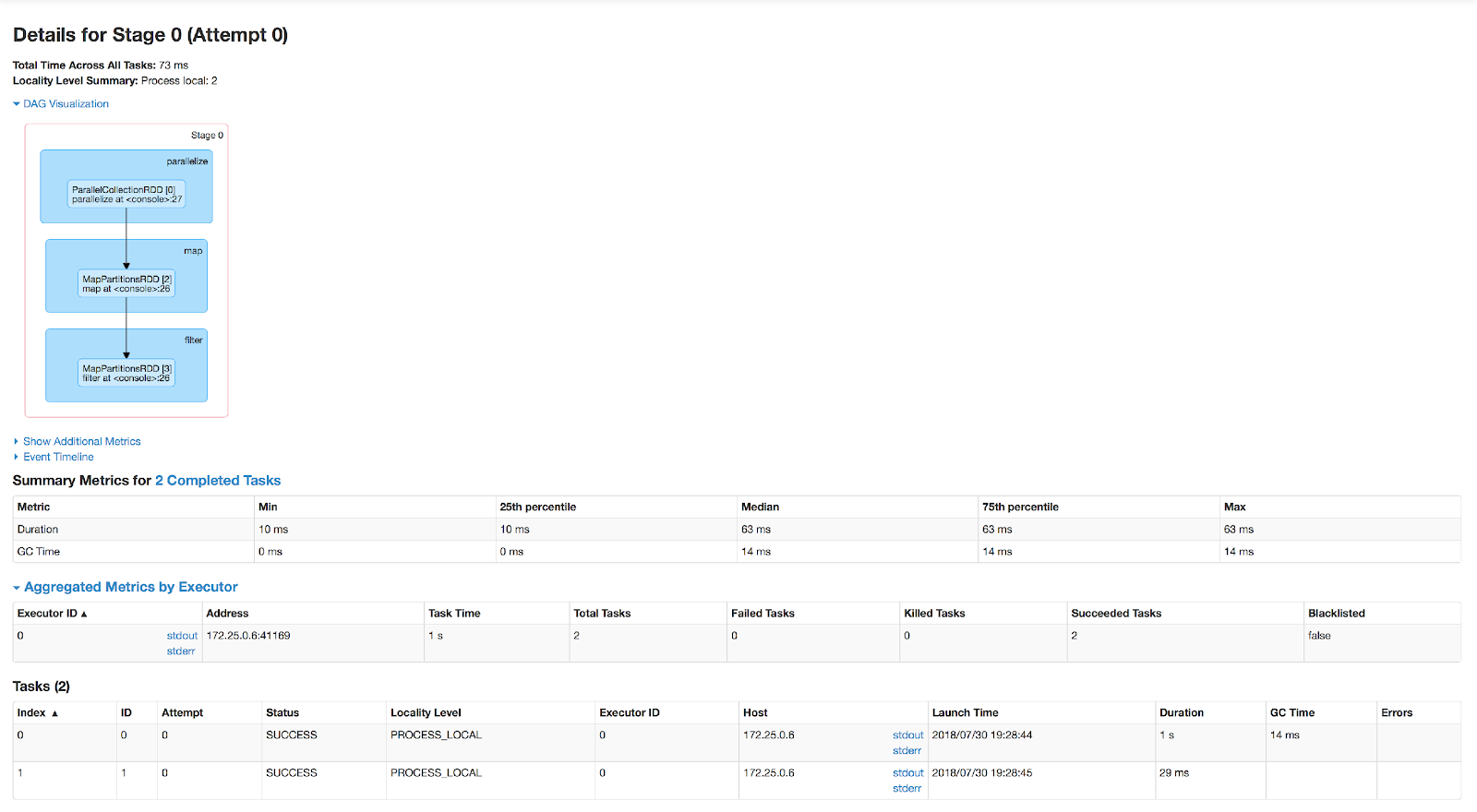
The DAG visualization in this view shows the runtime type of every intermediate RDD produced by the stage and the line at which it was defined. Apart from that, there’s yet another term on this page – a task. A task represents the execution of the transformations of all the nodes in the DAG on one of the partitions of the RDD.

Concretely, can be thought of as the composition of all the transform: Iterator[T] => Iterator[U] functions we saw before.

You’ll note that the Tasks table at the bottom lists two tasks. This is due to the RDD consisting of two partitions; generally, every transformation will result in a task for every partition in the RDD. These tasks are executed on the executors of the cluster. Every task runs in a single thread and can run in parallel with other tasks, given enough CPU cores on the executor.

So, to recap, we have:

• jobs, which represent a full data transformation execution triggered by an action;
• stages, which we have not defined yet;
• tasks, each of which represents the execution of a transform: Iterator[T] => Iterator[U] function on a partition of the RDD.

To demonstrate what stages are, we’ll need a more complex example:

Here, we create two RDDs representing the employee and department tables (in tribute to the venerable SCOTT schema); we group the employees by department ID, join them to the department RDD, sum the salaries in each department and collect the results into an array.

collect is an action, so by executing it, we have initiated a job. You should be able to locate it in the Jobs tab in the UI, and click its description; the DAG on the detail page should look similar to this:

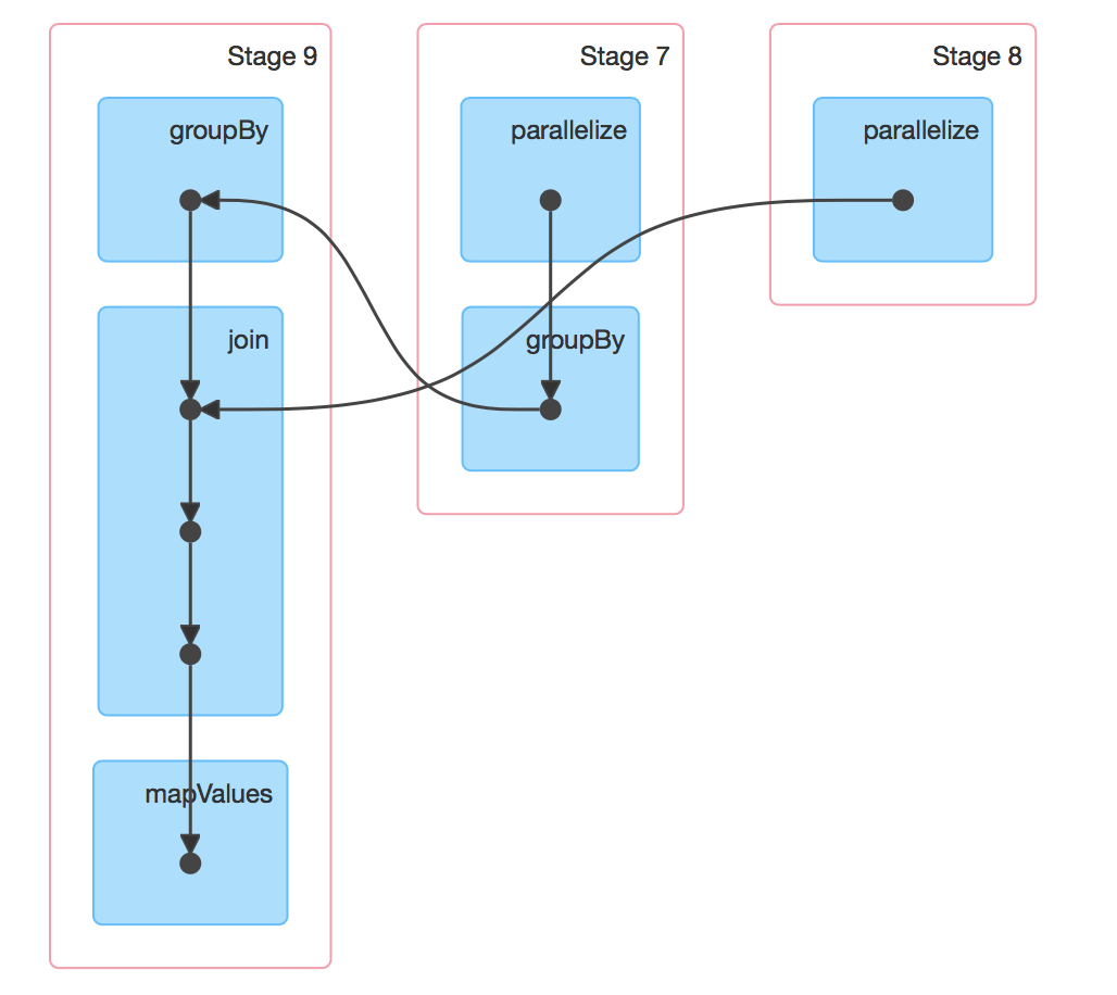
This is much more interesting! We now have 3 stages instead of a single stage, with the two smaller ones funneling into the larger one. Stage 7 is the creation and grouping of the emp data, stage 8 is the creation of the dept data, and they both funnel into stage 9 which is the join and mapping of the two RDDs.

The horizontal order of the stages and their numbering might show up differently on your setup, but that does not affect the actual execution.

So, why is our job divided into three stages this time? The answer lies with the type of transformations that comprise the job.

If you recall, we discussed narrow and wide transformations in the previous post. Narrow transformations – such as map and filter – do not move rows between RDD partitions. Wide transformations, such as groupBy require rows to be moved. Stages are in fact bounded by wide transformations (or actions): a stage groups transformations that can be executed on the same worker without data shuffling.

A shuffle is the process in which rows are exchanged between the RDD partitions and consequently between workers. Note what happens in this visualization of the groupBy transformation:

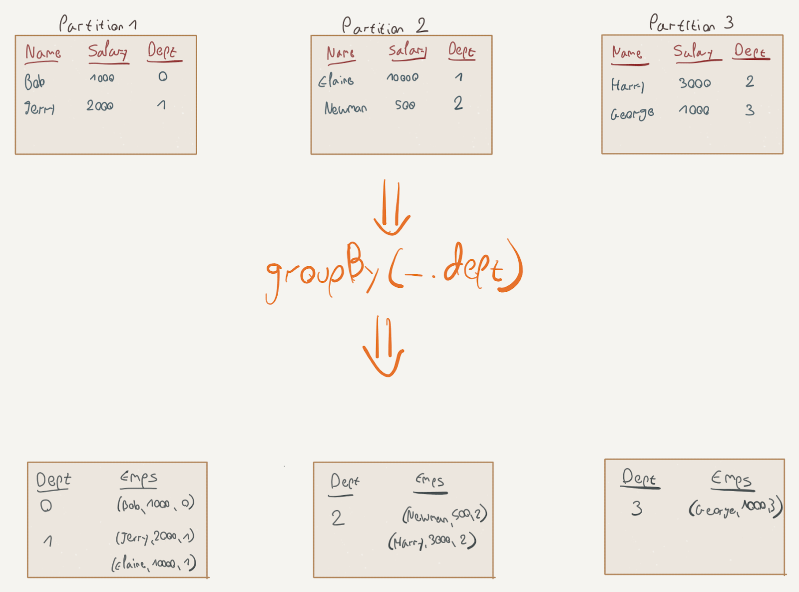
The elements for the resulting key were scattered across several partitions and now need to be shuffled into one partition. The stage boundary is often also called the shuffle boundary; shuffling is the process in Spark in which elements are transferred between partitions.

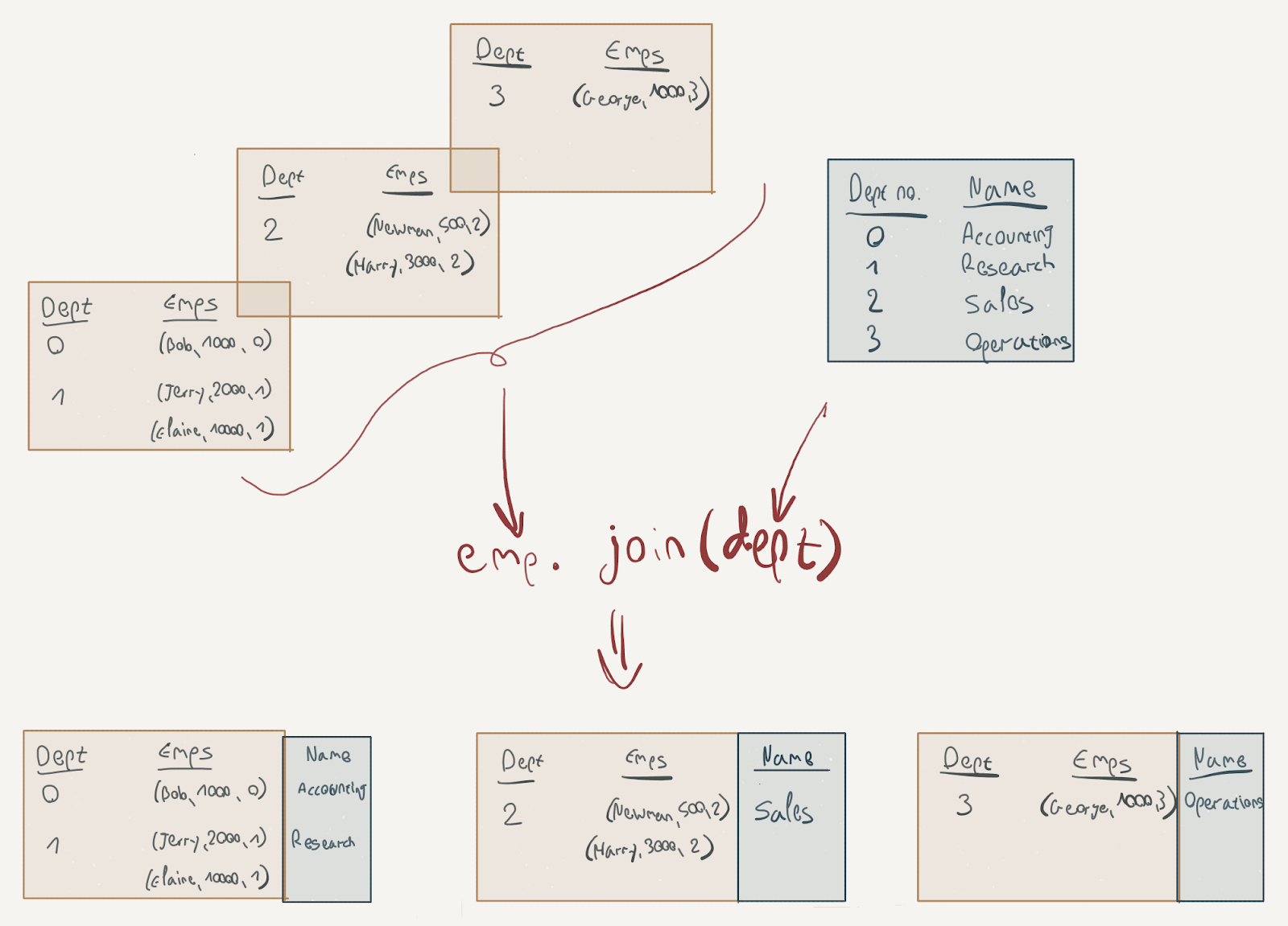
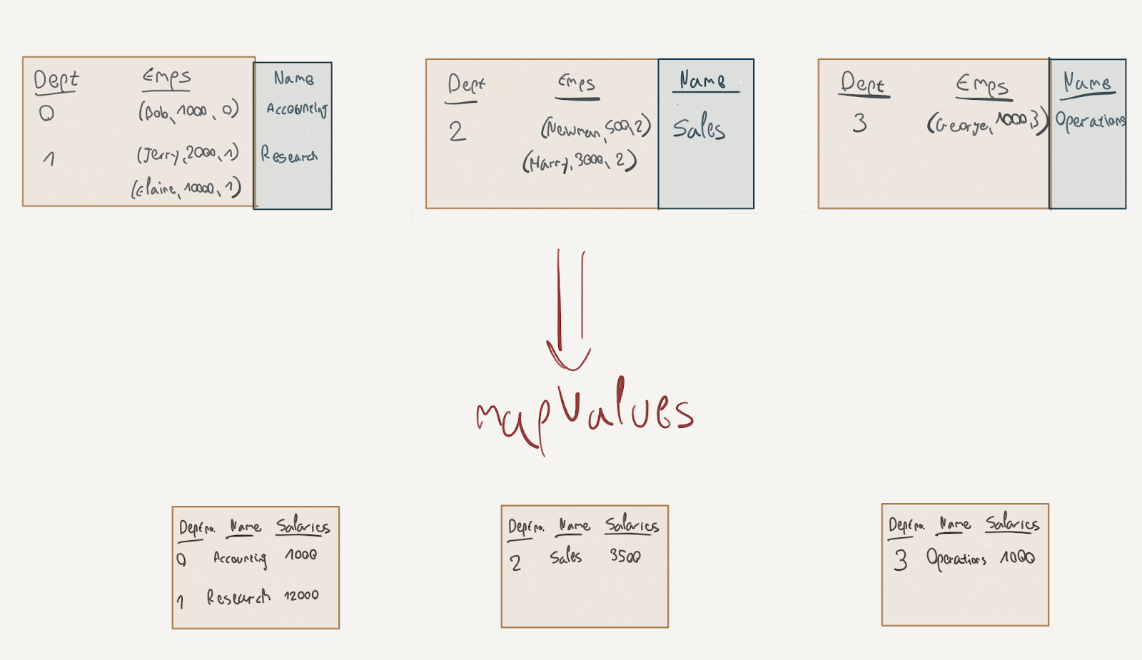
To complete the flow, here’s what happens after the groupBy stages; the join operation is a wide transformation as well, as it has to move data from the dept partition into the other partitions (this is a simplification, of course, as joining is a complicated subject) while the mapValues transformation is a narrow transformation:

Now that we know a bit more about the actual execution of our Spark jobs, we can further examine the architecture of the DataStax connector to see how it interacts with Scylla.

The DataStax Connector: A Deeper Look

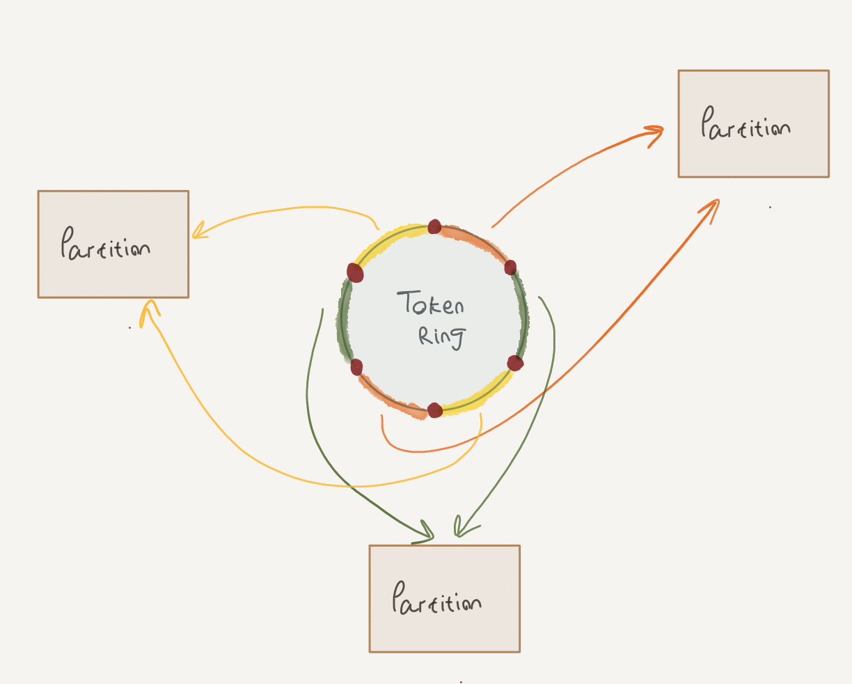
As we’ve discussed in the previous post, rows in Scylla tables are distributed in the cluster according to their partition keys. To describe this process briefly, every Scylla cluster contains a collection of number ranges that form a token ring. Every range is owned by one (or more, depending on the replication factor) of the cluster nodes.

When inserting a row to Scylla, the partition key is hashed to derive its token. Using this token, the row can be routed and stored in the right node. Furthermore, when processing table read requests that span several token ranges, Scylla can serve the data from multiple nodes.

In a way, this is similar to Spark’s concept of tasks and partitions; as Scylla tables are comprised of token ranges, RDDs are also comprised of partitions. Spark tasks process RDD partitions in parallel, while Scylla can process token ranges in parallel (assuming the relevant ranges are stored on different nodes).

Now, if we’re reading data from Scylla into RDD partitions and processing it in Spark tasks, it would be beneficial to have some alignment between the Scylla token ranges and the RDD partitions. Luckily for us, this is exactly how the DataStax connector is designed.

The logic for creating the RDD partitions is part of the RDD interface:

The RDD created by sc.cassandraTable contains the logic for assigning multiple token ranges to each partition – this is performed by the CassandraPartitionGenerator class.

First, the connector will probe Scylla’s internal system.size_estimates table to estimate the size, in bytes, of the table. This size is then divided by the split_size_in_mb connector parameter (discussed further below); the result will be the number of partitions comprising the RDD.

Then, the connector will split the token ranges into groups of ranges. These groups will end up as the RDD partitions. The logic for converting the groups into partitions is in TokenRangeClusterer, if you’re interested; the gist is that every group will be an equal portion of the token ring and that every group can be fetched entirely from a single node.

After the token range groups are generated, they can be converted to collections of CQL WHERE fragments that will select the rows associated with each range; here’s a simplified version of the fragment generated:

WHERE token(key) > rangeStart AND token(key) <= rangeEnd

The CqlTokenRange class that is stored on the partition reference on the RDD handles the fragment generation. The token function is a built-in CQL function that computes the token for a given key value; essentially, it hashes the value using the configured Scylla partitioner. You can read more about this approach to full table scans in this article.

When the stage tasks are executed by the individual executors, the CQL queries are executed against Scylla with the fragments appended to them. Knowing how this works can be beneficial when tuning the performance of your Spark jobs. In a later post in this series, we will show how to go through the process of tuning a misbehaving job.

The split_size_in_mb parameter we mentioned earlier controls the target size of each RDD partition. It can be configured through Spark’s configuration mechanism, using the --conf command line parameter to spark-shell:

Data and Closures

We’ve covered a fair bit about how Spark executes our transformations but glossed over two fairly important points. The first point is the way data in RDD partitions is stored on executors.

RDD Storage Format

For the initial task that reads from Scylla, there’s not much mystery here: the executors run the code for fetching the data using the DataStax driver and use the case class deserialization mechanism we showed in the last post to convert the rows to case classes.

However, later tasks that run wide transformations will cause the data to be shuffled to other executors. Moving instances of case classes over the wire to other machines doesn’t happen magically; some sort of de/serialization mechanism must be involved here.

By default, Spark uses the standard Java serialization format for shuffling data. If this makes you shudder, it should! We all know how slow Java serialization is. As a workaround, Spark supports using Kryo as a serialization format.

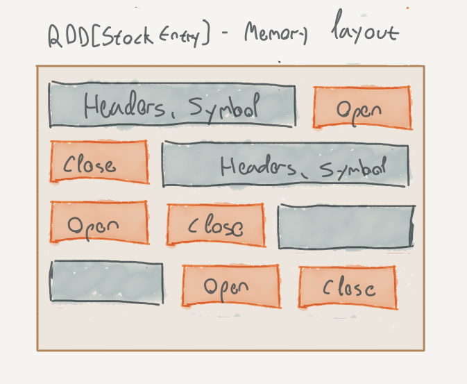
Apart from using Java serialization, there are other problems with naively storing objects in the executor’s memory. Consider the following data type:

Stored as a Java object, every StockEntry instance would take up:

• 12 bytes for the object header
• 4 bytes for the String reference
• 8 bytes for the integers

However, we also need to take into account the String itself:

• Another 12 bytes for the header
• 4 bytes for the char[] reference;
• 4 bytes for the computed hashcode
• 4 bytes for word boundary alignment

So that’s 48 bytes, not including the symbol string itself, for something that could theoretically be packed into 12 bytes (assuming 4 bytes for the symbol characters, ASCII encoded).

Apart from the object overhead, the data is also stored in row-major order; most analytical aggregations are performed in a columnar fashion, which means that we’re reading lots of irrelevant data just to skip it.

Closures

The second point we’ve glossed over is what Spark does with the bodies of the transformations. Or, as they are most commonly called, the closures.

How do those closures actually get from the driver to the executors? To avoid getting into too many details about how function bodies are encoded by Scala on the JVM, we’ll suffice in saying that the bodies are actually classes that can be serialized and deserialized. The executors actually have the class definitions of our application, so they can deserialize those closures.

There are some messy details here: we can reference outside variables from within our closure (which is why it is called a closure); do they travel with the closure body? What happens if we mutate them? It is best not to dwell on these issues and just avoid side-effects in the transformations altogether.

Lastly, working with closures forces us to miss out on important optimization opportunities. Consider this RDD transformation on the StockEntry case class, backed by a table in Scylla:

The result of this transformation is a map with the number of occurrences for each symbol. Note that we need, in fact, only the symbol column from the Scylla table. The query generated by the connector, however, tells a different story:

Despite our transformation only using symbol, all columns were fetched from Scylla. The reason being that Spark treats the function closures as opaque chunks of code; no attempt is done to analyze them, as that would require a bytecode analysis mechanism that would only be heuristic at best (see SPARK-14083 for an attempt this).

We could work around this particular problem, were it to severely affect performance, by using the select method on the CassandraTableScanRDD, and hinting to the connector which columns should be fetched:

This might be feasible in a small and artificial snippet such as the one above, but harder to generalize to larger codebases. Note that we also cannot use our StockEntry case class anymore, as we are forcing the connector to only fetch the symbol column.

To summarize, the biggest issue here is that Spark cannot “see” through our closures; as mentioned, they are treated as opaque chunks of bytecode that are executed as-is on the executors. The smartest thing that Spark can do to optimize this execution is to schedule tasks for narrow transformations on the same host.

These issues are all (mostly) solved by Spark SQL and the Dataset API.

Spark SQL and the Dataset API

Spark SQL is a separate module that provides a higher-level interface over the RDD API. The core abstraction is a Dataset[T] – again, a partitioned, distributed collection of elements of type T. However, the Dataset also includes important schema information and a domain-specific language that uses this information to run transformations in a highly optimized fashion.

Spark SQL also includes two important components that are used under the hood:

• Tungesten, an optimized storage engine that stores elements in an efficiently packed, cache-friendly binary format in memory on the Spark executors
• Catalyst, a query optimization engine that works on the queries produced by the Dataset API

We’ll start off by constructing a Dataset for our StockEntry data type backed by a Scylla table:

First, note that we are using the spark object to create the Dataset. This is an instance of SparkSession; it serves the same purpose as sc: SparkContext, but provides facilities for the Dataset API.

The cassandraFormat call will return an instance of DataFrameReader; calling load on it will return an instance of DataFrame. The definition of DataFrame is as follows:

type DataFrame = Dataset[Row]

Where Row is an untyped sequence of data.

Now, when we called load, Spark also inferred the Dataset’s schema by probing the table through the connector; we can see the schema by calling printSchema:

Spark SQL contains a fully fledged schema representation that can be used to model primitive types and complex types, quite similarly to CQL.

Let’s take a brief tour through the Dataset API. It is designed to be quite similar to SQL, so projection on a Dataset can be done using select:

Note how Spark keeps track of the schema changes between projections.

Since we’re now using a domain-specific language for projecting on Datasets, rather than fully fledged closures using map, we need domain-specific constructs for modeling expressions. Spark SQL provides these under a package; I recommend importing them with a qualifier to avoid namespace pollution:

The col function creates a column reference to a column named “open”. This column reference can be passed to any Dataset API that deals with columns; it also has functions named +, * and so forth for easily writing numeric expressions that involve columns. Column references are plain values, so you could also use a function to create more complex expressions:

If you get tired of writing f.col, know that you can also write it as $"col". We’ll use this form from now on.

Note that column references are untyped; you could apply a column expression to a dataset with mismatched types and get back non-sensical results:

Another pitfall is that using strings for column references denies us the compile-time safety we’ve had before; we’re awarded with fancy stack traces if we manage to mistype a column name:

The Dataset API contains pretty much everything you need to express complex transformations. The Spark SQL module, as it name hints, also includes SQL functionality; here’s a brief demonstration:

We can register Datasets as tables and then query them using SQL.

Check out the docs to learn more about the Dataset API; it provides aggregations, windowing functions, joins and more. You can also store an actual case class in the Dataset by using the as function, and still use function closures with map, flatMap and so on to process the data.

Let’s see now what benefits we reap from using the Dataset API.

Dataset API Benefits

Like every good database, Spark offers methods to inspect its query execution plans. We can see such a plan by using the explain function:

We get back a wealth of information that describes the execution plan as it goes through a series of transformations. The 4 plans describe the same plan at 4 phases:

• Parsed plan – the plan as it was described by the transformations we wrote, before any validations are performed (e.g. existence of columns, etc)
• Analyzed plan – the plan after it was analyzed against the schemas of the relations involved
• Optimized plan – the plan after optimizations were applied to it – we’ll see a few examples of these in a moment
• Physical plan – the plan after being translated to actual operations that need to be executed.

So far, there’s not much difference between the phases; we’re just reading the data from Scylla. Note that the type of the relation is a CassandraSourceRelation – a specialized relation that can interact with Scylla and extract schema information from it.

In the physical plan’s Scan operator, note that the relation lists all columns that appear in the table in Scylla; this means that all of them will be fetched. Let’s see what happens when we project the Dataset:

Much more interesting. The parsed logical plan now denotes symbol as an unresolved column reference; its type is inferred only after the analysis phase. Spark is many times referred to as a compiler, and these phases demonstrate how true this comparison is.

The most interesting part is on the physical plan: Spark has inferred that no columns are needed apart from the symbol column and adjusted the scan. This will cause the actual CQL query to only select the symbol column.

This doesn’t happen only with explicit select calls; if we run the same aggregated count from before, we see the same thing happening:

Spark figured out that we’re only using the symbol column. If we use max($"open") instead of count, we see that Spark also fetches the open column:

Being able to do these sort of optimizations is a very cool property of Spark’s Catalyst engine. It can infer the exact projection by itself, whereas when working with RDDs, we had to specify the projection hints explicitly.

As expected, this also extends to filters; we’ve shown in the last post how we can manually add a predicate to the WHERE clause using the where method. Let’s see what happens when we add a filter on the day column:

The PushedFilters section in the physical plan denotes which filters Spark tried to push down to the data source. Although it lists them all, only those that are denoted with a star (e.g. *LessThan(day,2010-02-01)) will actually be executed by Scylla.

This is highly dependent on the integration; the DataStax connector contains the logic for determining whether a filter would be pushed down or not. For example, if we add an additional filter on open, it would not be pushed down as it is not a part of the table’s primary key (and there is no secondary index on it):

The logic for determining which filters are pushed down to Scylla resides in the BasicCassandraPredicatePushDown class. It is well documented, and if you’re wondering why your predicate isn’t getting pushed down to Scylla, that would be a good place to start your investigation; in particular, the predicatesToPushdown member contains a set of all predicates determined to be legal to be executed by Scylla.

The column pruning optimization we discussed is part of a larger set of optimizations that are part of the Catalyst query optimization engine. For example, Spark will merge adjacent select operations into one operation; it will simplify boolean expressions (e.g. !(a > b) => a <= b), and so forth. You can see the entire list in org.apache.spark.sql.catalyst.optimizer.Optimizer, in the defaultBatches function.

Summary

In this post, we’ve discussed, in depth, how Spark physically executes our transformations, using tasks, stages, and jobs. We’ve also seen what problems arise from using the (relatively) crude RDD API. Finally, we’ve demonstrated basic usage of the Dataframe API with Scylla, along with the benefits we reap from using this API.

In the next post, we’ll turn to something we’ve not discussed yet: saving data back to Scylla. We’ll use this opportunity to also discuss the Spark Streaming API. Stay tuned!

Next Steps

• Scylla Summit 2018 is around the corner. Register now!
• Learn more about Scylla from our product page.
• See what our users are saying about Scylla.
• Download Scylla. Check out our download page to run Scylla on AWS, install it locally in a Virtual Machine, or run it in Docker.

The post Hooking up Spark and Scylla: Part 2 appeared first on ScyllaDB.

There’s nothing we enjoy more than celebrating the amazing things our users are accomplishing as a result of adopting Scylla. With that in mind, we’re excited to announce that nominations are now open for the first-annual Scylla User Awards.

Nominations will be accepted until September 28, 2018.

Nominate your company or project and we’ll send you a Scylla hoodie! Winners will be announced at Scylla Summit 2018. Oh, and award winners can attend the Scylla Summit at no cost!

Do you have an especially interesting Scylla use case? Is it pioneering in your industry? Does it benefit society? Or perhaps you’ve got a high number of concurrent users or lots of data centers. Have you been contributing to Scylla Open Source or reporting issues?

If so, please tell us all about yourself and your use case. Submit a valid nomination and we’ll send you a limited-edition Scylla hoodie in your size.

2018 Scylla User Award Categories:

• Most Interesting Technical Use Case
• Most Interesting Industry Use Case
• Best Use of Scylla as a Backend to an As-a-Service Offering
• Best Use of Scylla for Time Series
• Scylla Humanitarian Award
• Shortest Time from Download to Production
• Most Concurrent Users on a Scylla-based Application
• Most Data Centers Running Scylla
• Most Valuable Contribution(s) to Scylla Open Source
• Most Valuable (Community) Player
• Best Issue Reporter

You can nominate yourself in as many categories as you like. We look forward to seeing all the great things you’re doing with Scylla!

Next Steps

• Scylla Summit 2018 is around the corner. Register now!
• Learn more about Scylla from our product page.
• See what our users are saying about Scylla.
• Download Scylla. Check out our download page to run Scylla on AWS, install it locally in a Virtual Machine, or run it in Docker.

The post Introducing the First Annual Scylla User Awards appeared first on ScyllaDB.

When choosing a database solution it’s important to make sure it can scale to your business needs and provide fault tolerance and high availability. Scylla incorporates many features of Apache Cassandra’s scale-out design, including distributed workload and storage along with eventual consistency. In this post, we will explore how fault tolerance works and the high availability of Scylla’s architecture. This blog is meant for new users of Scylla. Advanced users are probably already familiar with these basic concepts (By the way, advanced users are also encouraged to nominate themselves for our Scylla User Awards).

What happens if a catastrophe occurs in or between your data centers? What if a node goes down or becomes unreachable for any reason? Scylla’s fault tolerance features significantly mitigate the potential for catastrophe. To get the best fault tolerance out of Scylla, you’ll need to understand how to select the right fault tolerance strategy, which includes setting a Replication Factor (the number of nodes that contain a copy of the data) for your keyspaces and choosing the right Consistency Level (the number of nodes that must respond to read or write operations).

Like many distributed database systems, Scylla adheres to the CAP Theorem: In a distributed system, consistency, availability, and partition tolerance of data are mutually dependent. Increasing (or decreasing) any 2 of these factors will inversely affect the third.

Scylla adheres to the CAP Theorem in the following way:

Scylla chooses availability and partition tolerance over consistency, such that:

• It’s impossible to be both consistent and highly available during a network partition
• If we sacrifice consistency, we can be highly available

Specifying a replication factor (RF) when setting up your Scylla keyspaces ensures that your keyspace is replicated to the number of nodes you specify. Since this affects performance and latency, your consistency level (CL) – tunable for each read and write query – lets you incrementally adjust how many read or write acknowledgments your operation requires for completion.

The replication factor and consistency level play important roles in making Scylla highly available. The Replication Factor (RF) is equivalent to the number of nodes where data (rows and partitions) are replicated. Data is replicated to multiple (RF=N) nodes. An RF of 1 means there is only one copy of a row in a cluster and there is no way to recover the data if the node is compromised or goes down. RF=2 means that there are two copies of a row in a cluster. An RF of at least 3 is used in most systems or similar.

Data is always replicated automatically. Read or write operations can occur to data stored on any of the replicated nodes.

In the example above, our client sends a request to write partition 1 to node V; 1’s data is replicated to nodes W, X, and Z. We have a Replication Factor (RF) of 3. In this drawing, V is a coordinator node but not a replicator node. However, replicator nodes can also be coordinator nodes, and often are.

During a read operation, the client sends a request to the coordinator. Effectively because the RF=3, 3 nodes respond to the read request.

The Consistency Level (CL) determines how many replicas in a cluster must acknowledge read or write operations before it is considered successful.
Some of the most common Consistency Levels used are:

• ANY – A write is written to at least one node in the cluster. Provides the highest availability with the lowest consistency.
• QUORUM – When a majority of the replicas respond, the request is honored. If RF=3, then 2 replicas respond. QUORUM can be calculated using the formula (n/2 +1) where n is the Replication Factor.
• ONE – If one replica responds, the request is honored.
• LOCAL_ONE – At least one replica in the local data center responds.
• LOCAL_QUORUM – A quorum of replicas in the local datacenter responds.
• EACH_QUORUM – (unsupported for reads) – A quorum of replicas in ALL data centers must be written to.
• ALL – A write must be written to all replicas in the cluster, a read waits for a response from all replicas. Provides the lowest availability with the highest consistency.

During a write operation, the coordinator communicates with the replicas (the number of which depends on the Consistency Level and Replication Factor). The write is successful when the specified number of replicas confirm the write.

In the above diagram, the double arrows indicate the write operation request going into the coordinator from the client and the acknowledgment being returned. Since the Consistency Level is one, the coordinator, V, must wait for the write to be sent to and responded by only a single node in the cluster, which is, in this case, W.

Since RF=3, our partition 1 is also written to nodes X and Z, but the coordinator does not need to wait for a response from them to confirm a successful write operation. In practice, acknowledgments from nodes X and Z can arrive to the coordinator at a later time, after the coordinator acknowledges the client.

When our Consistency Level is set to QUORUM, the coordinator must wait for a majority of nodes to acknowledge the write before it is considered successful. Since our Replication Factor is 3, we must wait for 2 acknowledgments (the third acknowledgment does not need to be returned):

During a read operation, the coordinator communicates with just enough replicas to guarantee that the required Consistency Level is met. Data is then returned to the client.

The Consistency Level is tunable per operation in CQL. This is known as tunable consistency. Sometimes response latency is more important, making it necessary to adjust settings on a per-query or operation level to override keyspace or even data center-wide consistency settings. In other words, the Consistency Level setting allows you to choose a point in the consistency vs. latency tradeoff.

The Consistency Level and Replication Factor both impact performance. The lower the Consistency Level and/or Replication Factor, the faster the read or write operation. However, there will be less fault tolerance if a node goes down. The Consistency Level itself impacts availability. A higher Consistency Level (more nodes required to be online) means less availability with less tolerance to tolerate node failures. A lower Consistency Level means more availability and more fault tolerance.

In this post, we went over Scylla’s highly-available architecture and explained fault tolerance. For more information on these topics, I encourage you to read our architecture and fault tolerance documentation.

Next Steps

• Scylla Summit 2018 is around the corner. Register now!
• Learn more about Scylla from our product page.
• See what our users are saying about Scylla.
• Download Scylla. Check out our download page to run Scylla on AWS, install it locally in a Virtual Machine, or run it in Docker.

The post A Beginner’s Guide to Scylla Fault Tolerance appeared first on ScyllaDB.

We’re pleased to announce that ScyllaDB is a diamond sponsor at the upcoming Distributed Data Summit – Apache Cassandra and Friends in San Francisco on September 14th. We’re excited to be part of this event, which brings together the top Apache Cassandra leaders and practitioners for one day of technical sessions. Like all Global Data Geeks events, you can also expect time for networking (and free drink tickets) at Happy Hour!

Interested in attending? Our diamond sponsorship includes a half-price discount for our guests, so use this link to save 50% off your registration, or apply this code when ordering through Eventbrite: “friend-of-scylladb-50”.

ScyllaDB CEO Dor Laor and CTO Avi Kivity will each give talks at the summit, plus Yahoo! Japan will present on their use of Cassandra and Scylla. Here is an overview of those sessions:

Cassandra and ScyllaDB at Yahoo! Japan
Shogo Hoshii – Yahoo! Japan
Murukesh Mohanan – Yahoo! Japan
Yahoo! JAPAN is one of the most successful internet service companies in Japan. Shogo will introduce his company’s business and its scale. He will go on to discuss the number of Cassandra nodes and clusters, and what kind of data is stored in them. He will go on to introduce some of the incidents that happened with the company’s Cassandra implementation, and how they managed to handle them. Murukesh Mohanan will go on to discuss the Yahoo! Japan NoSQL Team’s evaluation of ScyllaDB as a successor of Cassandra in exceedingly heavy traffic.

OLTP or Analytics? Why not both?
Avi Kivity – ScyllaDB
OLTP and Analytics are very different. One is characterized by many concurrent small requests, with a high sensitivity to latency, while the other typically processes large streams of data with more emphasis on throughput.
Avi’s talk will cover:

• The different requirements of the two workloads
• How ScyllaDB optimizes for both
• Performance isolation of different workloads within ScyllaDB
• How ScyllaDB supports concurrent OLTP and Analytics without sacrificing either latency or throughput
• Measurements

Shard per core vs threads in databases
Avi Kivity – ScyllaDB
This talk will cover the shard-per-core architecture of Scylla and compare it to the traditional threaded design employed by Cassandra. The recent adoption of thread-per-core by Datastax is further evidence of the gains this architecture offers over a threaded design. We will discuss the various design decisions that make a shard-per-core design ideal and how to tackle the architecture issues that come with it.

Was Cassandra the right baseline for ScyllaDB?
Dor Laor – ScyllaDB
The ScyllaDB team has been re-implementing Cassandra in C++ for the past 4 years, but was Cassandra the right baseline? Sure, Cassandra has hundreds of people years behind it and design wins that other frameworks can only imagine, but there are caveats too. If you follow the rest of the industry, from multi-tenant CosmosDB to transactional CockroachDB there’s a lot going on. Even within the Cassandra community there are different voices around sidecar management processes.
It’s a good time to take a step back and consider whether it was right to embrace the Cassandra design and APIs versus starting from a clean slate. This talk will cover programming language choices (Java, Go, C++), the use of existing engines (RocksDB), implementation of secondary indexes and management consoles, and more.

Summit Details
Distributed Data Summit – Apache Cassandra and Friends
Register and save 50%
Mission Bay Conference Center
1675 Owens Street
San Francisco, CA 94158
Friday, September 14, 2018 from 8:00 AM to 8:00 PM (PDT)

We hope to see you there! Stop by our booth to talk about your real-time big data projects, see a demo of Scylla, pick up swag and get some free drink tickets.

Next Steps

• Scylla Summit 2018 is around the corner. Register now!
• Learn more about Scylla from our product page.
• See what our users are saying about Scylla.
• Download Scylla. Check out our download page to run Scylla on AWS, install it locally in a Virtual Machine, or run it in Docker.

The post See Us at Distributed Data Summit 2018 appeared first on ScyllaDB.

In June, Miguel Martinez Pedreira, Software engineer at CERN on the ALICE project, and Glauber Costa, VP of Field Engineering at ScyllaDB, teamed up to do a computing seminar to discuss real-time processing of big data with ScyllaDB, examining how Scylla helped the ALICE experiment with their AliEn Global File Catalogue use case.

CERN uses the world’s largest and most complex scientific instruments to study the basic constituents of matter – the fundamental particles. The instruments used at CERN are purpose-built particle accelerators and detectors. Accelerators boost beams of particles to high energies before the beams collide with each other or with stationary targets. This process that gives physicists insights into the fundamental laws of nature.

One of seven experiments on CERN’s Large Hadron Collider, ALICE (A Large Ion Collider Experiment) studies the hadrons, electrons, muons and photons produced in the collisions of heavy nuclei. In the process, it creates matter at temperatures that exceed five trillion Kelvins, about 333,000 times hotter than the core of the sun.

The AliEn Global File Catalogue is a metadata index of every single file of the experiment. It spreads across 80 computer centers in five continents. The real-time data is stored from the moment it’s taken in the experiment, and made available for other phases of research.

See CERN and ScyllaDB present their Global File Catalogue use case of real-time processing along with the results of switching from Cassandra to Scylla in the video below. Glauber explains how Scylla enabled CERN to achieve high throughput at predictably low latencies, all while keeping TCOs under tight control.

Watch the video to learn about Scylla’s close-to-the-hardware architecture and how it helped CERN amp up their Global File Catalogue platform. You might also like to watch CERN’s presentation at Scylla Summit 2017, A Future-Proof Global File Catalogue for the ALICE Experiment at CERN.

The post CERN on Real-Time Processing of Big Data with Scylla appeared first on ScyllaDB.

Scylla Summit is the event we host every year where you can learn from your industry-leading colleagues, find out the latest in our technology vision and roadmap, and share your own ideas and opinions on what’s important to you and where we should take Scylla next.

You want to get the most out of your database instances. At Scylla Summit 2018, learn everything you need to know from our team and your peers about overcoming scaling issues, getting the lowest-possible latencies, and ensuring you run your database operations with the highest availability.

REGISTER NOW! Use the code BLOG50 to get 50% the current price of the 2-day pass.

Scylla Summit 2018 is where you can learn in detail how others have already successfully integrated Scylla into their own heterogeneous production environments. From developers using leading languages like C++, Python, or Golang. From architects combining Scylla with other NoSQL database systems. And from DevOps integrating it with Spark, Kafka, Kubernetes and more.

At this, our third Scylla Summit, you’ll have the opportunity to:

• Attend one of our pre-summit training tracks (both for Beginners and Advanced) on November 5, conducted by ScyllaDB’s lead engineers and the one-and-only Avi Kivity, our CTO and co-founder
• See how others use Scylla at scale and learn about innovative use cases
• Learn how to build next-generation applications with enormous scale by developing client code for unmatched low latency and high performance
• Take a deep dive into Scylla’s integrations with Spark and Kafka, and analyze them down to the closure, shard and table levels (For a preview example, see our recent blog series on Hooking up Spark and Scylla)
• Understand how Kubernetes and Scylla can complement each other
• Optimize your deployment with the right choice of materialized views, secondary indexes, and filtering
• Get new insights into our roadmap. This is critical. We need your opinions and requirements to help steer our product direction for 2019 and beyond
• Understand the fundamentals of the Seastar engine, and how we go from basic schedulers to combining OLTP and OLAP workloads on the same nodes

The Scylla community has experienced tremendous growth over the last year. Our database has been adopted and put into production by leading organizations across a number of industries and use cases. Whether in travel, AdTech, automotive, manufacturing, or industrial IoT, you will find Scylla instances providing real-time recommendations, giving marketers 360º customer views, ingesting live data from fleets of vehicles and more. I’m sure you will find these use cases fascinating, as well as the conversations with our staff and your peers at our networking events.

Whether you are a current Scylla community member, user, or developer, or you have a background with Cassandra, NoSQL or other database technologies and are eager to learn more, I’d like to invite you personally to join us, this November 6th and 7th, at the Pullman Hotel, Redwood City, in the San Francisco Bay Area, near SFO, and convenient to San Francisco, Silicon Valley, and all points in between.

As a last note: though the official call for speakers has closed, we are always interested in hearing of your successes and breakthroughs. If you have a unique use case for Scylla you want to share, and we haven’t heard about it yet, you can still submit your abstract here.

Best,

Dor

The post Scylla Summit 2018: For Our Event-Driven Engineers appeared first on ScyllaDB.

Large partitions, although supported by Scylla, are also well known for causing performance issues. Fortunately, release 2.3 comes with a helping hand for discovering and investigating large partitions present in a cluster — system.large_partitions table.

Large partitions

CQL, as a data modeling language, aims towards very good readability and hiding unneeded implementation details from users. As a result, sometimes it’s not clear why a very simple data model suffers from unexpected performance problems. One of the potential suspects might be large partitions. Our blog entry on large partitions contains a detailed explanation on why coping with large partitions is important. We’ll use some of the same example tables from this article below.

The following table could be used in a distributed air quality monitoring system with multiple sensors:

CREATE TABLE air_quality_data (
   sensor_id text,
   time timestamp,
   co_ppm int,
   PRIMARY KEY (sensor_id, time)
);

With time being our table’s clustering key, it’s easy to imagine that partitions for each sensor can grow very large – especially if data is gathered every couple of milliseconds. Given that there is a hard limit on the number of clustering rows per partition (2 billion) this innocent looking table can eventually become unusable. In this example, in about 50 days.

A standard solution is to amend the data model to reduce the number of clustering keys per partition key. In this case, let’s take a look at amended table air_quality_data:

CREATE TABLE air_quality_data (
   sensor_id text,
   date text,
   time timestamp,
   co_ppm int,
   PRIMARY KEY ((sensor_id, date), time)
);

After the change, one partition holds the values gathered in a single day, which makes it less likely to overflow.

system.large_partitions table

Amending the data model may help with large partition issues. But sometimes you have such issues without realizing it. It’s useful to be able to see which tables have large partitions and how many of them exist in a cluster.

In order to track how many large partitions are created and to which table they belong, one can use the system.large_partitions table, which is implicitly created with the following schema:

CREATE TABLE system.large_partitions (
keyspace_name text,
table_name text,
sstable_name text,
partition_size bigint,
partition_key text,
compaction_time timestamp,
PRIMARY KEY ((keyspace_name, table_name), sstable_name, partition_size, partition_key)
) WITH CLUSTERING ORDER BY (sstable_name ASC, partition_size DESC, partition_key ASC);

How it works

Partitions are written to disk during memtable flushes and compaction. If, during any of this action, a large partition is written, an entry in system.large_partitions will be created (or updated). It’s important to remember that large partition information is updated when a row is actually written to disk; changes might not be visible immediately after acknowledging a write operation by the user, since data could still reside in a memtable for some time.

Each entry in system.large_partitions table represents a partition written to a given sstable. Note that large_partitions table is node-local – querying it will return large partition information only for the node that serves the request.

Listing all local large partition info can be achieved with:

SELECT * FROM system.large_partitions;

Checking large partitions for a specific table:

SELECT * FROM system.large_partitions WHERE keyspace_name = 'ks' and table_name = 'air_quality_data';

Listing all large partitions in a given keyspace that exceeded 140MB:

SELECT * FROM system.large_partitions WHERE partition_size > 146800640 ALLOW FILTERING; *

• Note: ALLOW FILTERING support is not part of 2.3; it will be present in the next release

Listing all large partitions compacted today:

SELECT * FROM system.large_partitions WHERE compaction_time >= toTimestamp(currentDate()) ALLOW FILTERING; *

• Note: ALLOW FILTERING support is not part of 2.3; it will be present in the next release

Since system.large_partitions can be read just like a regular CQL table, there are many more combinations of queries that return helpful results. Remember that keyspace_name and table_name act as the partition key, so some more complex queries, like the last example above, may involve filtering (hence the appended ALLOW FILTERING keywords). Filtering support for such queries is not part of 2.3 and will be available in the next release.

Aside from table name and size, system.large_partitions contains information on the offending partition key, when the compaction that led to the creation of this large partition occurred, and its sstable name (which makes it easy to locate its filename).

Configuration

For both readability and performance reasons, not all partitions are registered in system.large_partitions table. The threshold can be configured with an already existing parameter in scylla.yaml:

compaction_large_partition_warning_threshold_mb: 100

Previously, this configuration option was used to trigger a warning and logged each time a large-enough partition was written.

The large partition warning threshold defaults to 100MiB, which implies that each larger partition will be registered into system.large_partitions table the moment it’s written, either because of memtable flush or as a result of compaction.

If the default value is not sufficient for a specific use case, e.g. even 1MiB partitions are considered “too big” or, conversely, virtually every partition is bigger than 100MiB, it you can modify compaction_large_partition_warning_threshold_mb accordingly.

Disabling system.large_partitions can effectively be done by setting the threshold to an extremely high value, say, 500GiB. However, it’s highly recommended to leave it at a reasonable level. Better safe than sorry.

In order to prevent stale data from appearing in system.large_partitions, each record is inserted with time-to-live of 30 days.

Conclusion

We promised back in 2016 for Release 1.3 that we’d continue to improve support for large partitions. This improvement for 2.3 is a follow-through on that commitment. As you can see, we already have some next-steps planned out with future support for ALLOW FILTERING.

For now, we’d like for you to try system.large_partitions, and let us know what you find. Are you already aware of large partitions in your database, or did it help you discover anything about your data you didn’t already know?

If large partitions are critical to you, feel free to contact us with your war stories and requirements, or bring them up when you see us at Scylla Summit this November.

The post Large Partitions Support in Scylla 2.3 and Beyond appeared first on ScyllaDB.

The post Scylla Summit Preview: Keeping Your Latency SLAs No Matter What! appeared first on ScyllaDB.

The Scylla team is pleased to announce the release of Scylla 2.3, a production-ready Scylla Open Source minor release.

The Scylla 2.3 release includes CQL enhancements, new troubleshooting tools, performance improvements and more. Experimental features include Materialized Views, Secondary Indexes, and Hinted Handoff (details below). Starting from Scylla 2.3, packages are also available for Ubuntu 18.04 and Debian 9.

Scylla is an open source, Apache Cassandra-compatible NoSQL database, with superior performance and consistently low latency. Find the Scylla 2.3 repository for your Linux distribution here.

Our open source policy is to support only the current active release and its predecessor. Therefore, with the release of Scylla 2.3, Scylla 2.2 is still supported, but Scylla 2.1 is officially retired.

Related Links     

• Get Scylla 2.3
• Upgrade from Scylla 2.2 to Scylla 2.3
• Report a problem

New Distribution Support

Scylla packages are now available for:

• Debian 9 #2541
• Ubuntu 18.04 #3598

AWS – Scylla AMI

The Scylla 2.3 AMI is now optimized for i3.metal as well. Read more on the performance gains of using bare-metal i3.metal compared to virtualized i3.16xlarge.

Tooling

• CQL: Identify Large Partitions. One of the common anti-patterns in Scylla is large partitions. Recent releases addressed this issue and the handling of large partitions was greatly improved. However, we still had to solve issues where reading a large partition is less efficient and does not scale as well. With this release, Scylla now identifies large partitions and makes the information available in a system table. This allows you to identify large partitions, giving you the ability to fix them. The threshold for large partitions can be set in scylla.yaml:

compaction_large_partition_warning_threshold_mb parameter (default 100MB)

Example:  SELECT * FROM system.large_partitions;

> More on large partitions support in scylla 2.3

• CQL Tracing: Added prepared statement parameters #1657
• Scyllatop – The Scyllatop tool, originally introduced with the Scylla Collectd API, is now using the Scylla Prometheus API, same as the Scylla Monitoring Stack. Starting from Scylla 2.3, Collectd is not installed by default, but the Collectd API is still supported.  #1541 #3490
• iotune v2. Iotune is a storage benchmarking tool that runs as part of the scylla_setup script. Iotune runs a short benchmark on the Scylla storage and uses the results to set the Scylla io_properties.yaml configuration file (formerly called io.conf). Scylla uses these settings to optimize I/O performance, specifically through setting max storage bandwidth and max concurrent requests.The new iotune output matches the new IO scheduler configuration, is time-limited (2 minutes) and produces more consistent results than the previous version.
• Python re-write: All scripts, previously written in bash, such as scylla_setup, were re-written in Python. This change does not have any visible effect but will make future enhancements easier.  See Google Bash Style Guide on the same subject.

New Features in Scylla 2.3

• CQL: Datetime Functions Support. Scylla now includes support for the following functions:

timeuuidtodate
timestamptodate
timeuuidtotimestamp
datetotimestamp
timeuuidtounixtimestamp
timestamptounixtimestamp
datetounixtimestamp

Example: SELECT * FROM myTable WHERE date >= currentDate() - 2d
#2949

• CQL: JSON Function Support: Scylla now includes support for: JSON operations, SELECT JSON, INSERT JSON, and the functions: toJson() and fromJson(). It is compatible with Apache Cassandra 2.2, with the exception of tuples and user-defined types. #3708Example:

CREATE TABLE test (
   a text PRIMARY KEY,
   b timestamp);

INSERT INTO test JSON '{  "a" : "Sprint", "b" : "2011-02-03 04:05+0000" }';

• CQL: Different timeouts for reads and range scans can now be set #3013
• CQL: TWCS support for using millisecond values in timestamps #3152 (used by KairosDB and others)
• Storage: Scylla now supports Apache Cassandra 2.2 file format (la sstable format). Native support for Apache Cassandra 3.0 file format is planned for the next major Scylla release.

Performance Improvements in Scylla 2.3

We continue to invest in increasing Scylla throughput and in reducing latency, focusing on reducing high percentile latencies.

• Dynamic controllers for additional compaction strategies. A dynamic controller for Size Tiered Compaction Strategy was introduced in Scylla 2.2. In Scylla 2.3, we have added controllers for Leveled Compaction Strategy and Time Window Compaction Strategy.
  
• Enhanced tagging for scheduling groups to improve performance isolation

Experimental Features

You are welcome to try the following features on a test environment. We welcome your feedback.

• Materialized Views (MV)
  With Scylla 2.3, MV is feature-compatible with Cassandra 3.0, but is not considered production ready. In particular, the following are part of the release:
  • Creating a MV based on any subset of columns of the base table, including the primary key columns
  • Updating a MV for base table DELETE or UPDATE.
  • Indexing of existing data when creating an MV
  • Support for MV hinted handoff
  • Topology changes, and migration of MV token ranges
  • Repair of MV tables
  • Sync of TTL between a base table and an MV table
  • nodetool viewbuildstatus

The following MV functions are not available in Scylla 2.3:

• • Backpressure – cluster may be overloaded and fail under a write workload with MV/SI – planned for the next release
  • Unselected columns keep MV row alive #3362, CASSANDRA-13826 – planned for the next release
  • MV on static and collection columns

• Secondary Indexes (SI)
  Unlike Apache Cassandra, Scylla’s SI is based on MV. This means every secondary index creates a materialized view under the hood, using all the columns of the original base table’s primary key, and the required indexed columns.The following SI functions are *not* available in Scylla 2.3:
  • Intersection between more than one SI and between an SI and a Partition Key – planned for the next release
  • Support for ALLOW FILTERING with a secondary index – planned for the next release
  • Paging support
  • Indexing of Static and Collection columns (same as for MV above)

• Hinted Handoff (see Scylla 2.2)

Metrics Updates from Scylla 2.2 to Scylla 2.3

• scylla Grafana Monitoring project now includes Scylla 2.3 dashboard on branch-1.0See here for all metrics changed in 2.3

Next Steps

• Scylla Summit 2018 is around the corner. Register now!
• Learn more about Scylla from our product page.
• See what our users are saying about Scylla.
• Download Scylla. Check out our download page to run Scylla on AWS, install it locally in a Virtual Machine, or run it in Docker.

The post Scylla Open Source Release 2.3 appeared first on ScyllaDB.

 

NoSQL practitioners from across the globe gathered this past Friday, 14 September 2018, in San Francisco for the latest Distributed Data Summit (#dds18). The attendees were as distributed as the data they manage, from the UK to Japan and all points between. While the event began years ago as a purely Apache Cassandra Summit, it currently bills itself as appealing to users of Apache Cassandra “and Friends.” The folks at ScyllaDB are definitely among those friends!

Spinning up for the event

Our team’s own efforts kicked off the night before with spinning up a 3-node cluster to show off Scylla’s performance for the show: two million IOPS with 4 ms latency at the 99.9% level. (And note the Average CPU Load pegged at 100%.)

A Hot Keynote

 

The keynote to the event was delivered by Nate McCall (@zznate), current Apache Cassandra Project Management Committee (PMC) Chair. He laid out the current state of Cassandra 4.0, including updates on its offerings, including Transient Replicas (14404) and Zero Copy Streaming (14556).

Nate acknowledged his own frustrations with Cassandra. For example, the “tick-tock” release model adopted in 2015, named after the practice originally promulgated by Intel. With a slide titled “Tick Toc Legacy: Bad,” Nate was pretty blunt, “I have to sacrifice a chicken [to get git to work].” Since Intel itself moved away from “tick-tock” in 2016, and the Cassandra community decided in 2017 to end tick-tock (coinciding with 3.10) in favor of 6-month release schedules, this is simply a legacy issue, but a painful one.

 

He also took a rather strident stance on Materialized Views, a feature Nate believes is not-quite-there-yet: “If you have them, take them out.”

 

When he mentioned the final nails in the coffin for Thrift (deprecated in favor of CQL), a hearty round of applause rose from the audience. Though, as an aside, Scylla will continue to support Thrift for legacy applications.

 

Nate also highlighted a number of sidecar proposals being made, such as The Last Pickle’s Cassandra Reaper for repairs, plus the Netflix and Datastax proposals.

 

Besides the specific technical updates, Nate also addressed maturity lifecycle issues that are starting to crop up in Cassandra. For the most part, he praised Cassandra staying close to its open source roots: “The features that are coming out are for users, by users… The marketing team is not involved.” But like Hadoop before it (which was split between Cloudera, Hortonworks and MapR), Cassandra is now witnessing increased divergence emerging between commercial vendors and code committers (such as DataStax and ScyllaDB).

Yahoo! Japan

The ScyllaDB team also had a chance to meet our friends Shogo Hoshii and Murukesh Mohanan. They presented on Cassandra and ScyllaDB at Yahoo! Japan, focusing on the evaluation they performed for exceedingly heavy traffic generated by their pre-existing Cassandra network of 1,700 nodes. Yahoo! Japan is no stranger to NoSQL technology, forming their NoSQL team in 2012. We hope to bring you more of their analyses and results in the future. For now, we’ll leave you with this one teaser slide Dor took during their presentation.

 

Was Cassandra the Right Base for Scylla?

ScyllaDB CEO Dor Laor asked this fundamental question for his session. If we knew then what we know now, four years ago, would we have still started with Cassandra as a base?

 

While Scylla mimics the best of Cassandra, it was engineered in C++ to avoid some of the worst of its pitfalls, such as JVM Garbage Collection, making it quite different under the hood.

 

Dor observed first “what worked well for us?” Particularly, inheriting such items as CQL, drivers, and the whole Cassandra ecosystem (Spark, KairosDB, JanusGraph, Presto, Kafka). Also, Cassandra’s “scale-out” capabilities, high availability and cross-datacenter replication. Backup and restore had reasonable solutions. (Though it is particularly nice to see people write Scylla-specific backup tools like Helpshift’s Scyllabackup.) Cassandra also has a rich data model, with key-value and wide rows. There was so much there with Cassandra. “Even hinted handoffs.” And, not to be left out of the equation, tools like Prometheus and Grafana.

 

On the other hand, there was a lot that wasn’t so great. Nodetool and JMX do not make a great API. The whole current sidecar debate lays bare that there was no built-in management console or strategy. Configurations based on IP are problematic. Dor’s opinion is that they should have been based on DNS instead. Secondary indexes in Cassandra are local and do not scale. “We fixed it” for Scylla, Dor noted.

 

Since 2014, a lot has changed in the NoSQL world. Dor cited a number of examples, from CosmosDB, which is multi-model and fully multi-tenant, to Dynamo’s point-in-time backups and streams, to CockroachDB’s ACID guarantees and SQL interface. Some of those features are definitely compelling. But would they have been a better place to start from?

 

So Dor took the audience on a step-by-step review of the criteria and requirements for what the founding team at ScyllaDB considered when choosing a baseline database.

 

Fundamental reliability, performance, and the ecosystem were givens for Cassandra. So those became quick checkboxes.

 

Dor instead focused on the next few bullets. Operational management could be better. Had it been part of Cassandra’s baseline, it would have obviated the need for sidecars.

 

For data and consistency, Dor cited Baidu’s use of CockroachDB for management of terabytes of data with 50 million inserts daily. But while that sounds impressive, a quick bit of math reveals that only equates to 578 operations per second.

 

While SSTables 3.0 provide a significant storage savings compared to 2.0, where Cassandra needs to improve in terms of storage and efficiency is to adopt a tiered-storage model (hot vs. cold storage).

 

“Cloud-native” is a term for which a specific definition is still quite arguable, especially when it comes to databases. Though there have been a few good takes at the topic, the term itself can still mean different things to different people, never mind the implementations. For instance, Dor brought up the example of what might happen if a split-brain divides the database and your Kubernetes (“k8s”) differently. Dor argued that Scylla/Cassandra’s topology awareness is better than Kubernetes, but the fact that they are different at all means there needs to be a reconciliation to heal the split-brain.

 

With regards to multi-tenancy, Dor saw the main problem here as one of idle resources, exacerbated by cloud vendors all-too-happy to over-provision. The opportunity here is to encapsulate workloads and keyspaces per tenant, and to provide full isolation, including system resources (CPU, memory, disk, network), security, and so on — without over-provisioning, and also while handling hot partitions well. It would require a single cluster for multiple tenants, consolidating all idle resources. Ideally, such a multi-tenant cluster would permit scale-outs in a millisecond. Dor also emphasized that there is a great need to define better SLAs that focus on real customer workloads and multi-tenancy needs.

 

So was Cassandra the right baseline to work from? Those who attended definitely got Dor’s opinion. But if you couldn’t attend, don’t worry! We plan on publishing an article delving into far more depth on this topic in the near future.

Thread per Core

 

ScyllaDB CTO Avi Kivity flew in from Israel to present on Scylla’s thread-per-core architecture.

 

The background to his talk was the industry momentum towards ever-increasing core counts. Utilizing these high core count machines is getting increasingly more difficult. Lock contention. Optimizing for NUMA and NUCA. Asymmetric architectures, which can lead to over- or under-utilization extremes.

 

Yet there are compelling reasons to deal with such difficulties to achieve significant advantages. Lowered mean time between failures (MTBFs) and reduced management burdens by dealing with orders of magnitude fewer machines. The use of far less space in your rack. Less switch ports. And, of course, a reduction in overall costs.

 

So, Avi asked, “How do you get the most from a large fat node?” Besides system architecture, there are also considerations within the core itself. “What is the right number of threads” to run on a single core? If you run too few, you can end up with underutilization. If you run too many, you run into the inverse problems of thrashing, lock contention and high latencies.

The natural fit for this issue is a thread-per-core approach. Data has traditionally been partitioned across nodes. This simply drills the model down to a per-core basis. It avoids all locking and kernel scheduling. And it scales up linearly. However, if you say “no kernel scheduling,” you have to take on all scheduling yourself. And everything has to be asynchronous.

In fact, each thread has to be able to perform all tasks. Reads. Writes. Compactions. Repairs. And all administrative functions. The thread also has to be responsible for balancing CPU utilization across these tasks, based on policies, and with sufficient granularity. Thus, the thread has to be able to preempt any and every task. And, finally, threads have to work on separate data to avoid any locking—a true “shared-nothing” architecture.

Avi took us on a tour of a millisecond in a thread’s life. “We maintain queues of tasks we want to run.” This “gives us complete control of what we want to run next.” You’ll notice the thread maintains preemption and poll points, to occasionally change its behavior. Every computation must be preemptable at sub-millisecond resolution.

Whether you were in the middle of SSTable reads or writes, compactions, intranode partitioning, replicating data or metadata or mutating your mutable data structures, “Still you must be able to stop at any point and turn over the CPU.”

Being able to implement this low-level thread-per-core architecture brought significant advantages to Scylla. In one use case, it allowed the contraction from 120 Cassandra i3.2xl nodes to just three (3) i3.16xl nodes for Scylla. Such a reduction in nodes maintained the exact same number of cores, yet required significantly lower administrative overhead.

OLTP or Analytics? Why not Both?

In a second talk, Avi asked the question that has been plaguing the data community for years.

Can databases support parallel workloads with conflicting demands? OLTP workloads asks for the fastest response time, high cache utilization, and has a random access pattern. OLAP on the other hand has a batchy nature, latency is less important while throughput and efficient processing is paramount. The workload can scan large amount of data and access them once, thus the data shouldn’t be cached.

As Chad Jones of Deep Information Sciences quipped at his Percona Live 2016 keynote, “Databases can’t walk and chew gum at the same time.” He observed you can optimize databases for reads, or writes, but not both. At least, that was his view in 2016.

So how do you get a single system to provide both Online Transaction Processing (OLTP) and Online Analytical Processing (OLAP)? Avi noted that workloads can compete with each other. Writes, reads, batch workloads, and even internal maintenance tasks like compactions or repairs can all dominate a system if left to their own devices.

Prior practices with Cassandra have focused on throttling, configuring maximum throughput. But this has often been a manual tuning effort, which could leave systems idle at certain points, while being unable to shift system resources during peak activities.

Finally, after years of investment in foreground and background workload isolation Scylla is able to provide different SLA guarantee for the end-user workloads.

Avi took the audience through the low-level methods Scylla, built on the Seastar scheduler, can allow users to create new scheduling classes, and thus assign relative resource shares. For example, imagine a role defined as follows:

 

CREATE ROLE analytics

   WITH LOGIN = true

   AND SERVICE_LEVEL = { ‘shares’: 200 };

 
This would create an analytics role that would be constrained to a share of system resources. Note that the rule limits the analytics role to portion of the resources, however, this is not a hard cap. In case there are enough idle resources the analytics workload can go beyond its share and thus get the best of all worlds — utilization for OLAP and low latency for OLTP.

Avi then shared the results of two experiments, creating an oltp and analytics user to simulate performance under different scenarios. In the second more-realistic scenario, Avi outlined setting a latency-sensitive online workload that would consume 50% of CPU, versus a batch load with three times the thread count that would try to achieve as much throughput as it could get.

The results of his experiments were promising, the oltp workload continued to perform exactly as before, despite the 3X competing workload from analytics.

Having a single datacenter that handles operational and Spark (analytics) workload is a huge advance by Scylla. There is no more need to reserve an entire datacenter together with 1x-3x data duplication for Spark. If you want to hear more about this novel ability, we will be covering it at the Scylla Summit in November.

Looking Towards an Official Cassandra Sidecar, Netflix

Focusing on Cassandra itself, there were a number of very interesting talks. One in particular by the team at Netflix on “Looking towards an Official C* Sidecar.” They’ve kindly shared their slides after the event. Netflix is no stranger to sidecars, being the home of Priam (first committed to github in 2011), as well as sidecars for other services like Raigad for Elasticsearch and Prana. We at ScyllaDB have our own vision on a Scylla sidecar, in the form of Scylla Manager, but it is vital to hear the views of major stakeholders in the Cassandra community like Netflix. If you didn’t attend DDS18, this is definitely a talk to check out!

See You at Scylla Summit!

It was great to meet so many of you at Distributed Data Summit. Let’s keep those conversations going. We’re looking forward to seeing you at our own event coming up in November, Scylla Summit 2018. There will be hands-on training plus in-depth talks on a wide range of technical subjects, practical use cases, and lessons-learned by some of the industry’s leading practitioners. Don’t delay! Register today!

Don't delay! Register today for Scylla Summit!

The post Overheard at Distributed Data Summit 2018 appeared first on ScyllaDB.

The post Scylla Monitoring Stack 2.0 appeared first on ScyllaDB.

In the run-up to Scylla Summit 2018, we’ll be featuring our speakers and providing sneak peeks at their presentations. The second interview in this series is with ScyllaDB’s own Vlad Zolotarov.

Vladislav “Vlad” Zolotarov is one of our experts at getting the most out of Scylla, having written articles in the past about CQL tracing, tracing slow queries, securing your cluster, and using Hinted Handoffs. He will speak at the Scylla Summit in a talk entitled Scylla Got Slow! Using Tools, Talent, and Tracing to Find Out Why. He took the time to give a sneak peak into his upcoming session.

 

Outside of work, Vlad enjoys off-road biking and spending time with his family.

 

“Slow” can mean many things to many people. Latency or throughput, storage I/O, process cycle times like compactions, or a raft of low-level tweaks such as CPU scheduling. What specific aspects will you focus on in your talk?

 

In the context of this talk “slow” means unsatisfactory Scylla’s performance: either throughput or latency. We will start from that and will try to drill down trying to identify the possible reason for a slowdown. And reasons may vary from suboptimal OS-level configuration (networking, I/O, etc.) to bad Scylla practices.

 

Speed improvements can be found within the database, but also in the applications and ecosystem the database is connected to. Will you focus solely on inside-the-box analysis, or also on broader systemic troubleshooting?

 

We will start with analyzing the server’s state first. However tools Scylla provides allow detecting issues that are caused not only by problems on the server side but on the application side as well.

 

 

What are the go-to tools you have in your toolbox?

 

First of all Scylla Monitoring, which is a bunch of Grafana dashboards representing various metrics from Scylla cluster. This is what you always start with. In many cases this is where it ends too.

 

But if you need to drill down more you’ll eventually get to nodetool (statistics commands), system log, cqlsh and CQL Tracing.

 

If you had a single, specific tip to give to Scylla database managers to improve performance, what would it be?

 

Always try to understand what the problem is before trying to fix anything. Remember that the cluster is going to work as fast as the slowest node and in Scylla’s case — as the slowest shard. Therefore always start with identifying where the bottleneck is. There are a few ways of approaching this, and we’ll discuss various methods during the talk.

Do you have any recommendations for Scylla Summit attendees of articles or topics they should review prior to when they sit down to hear you speak?

 

I expect people to know Scylla fundamentals and have a basic understanding of how a server like Scylla or Cassandra works: what is a cluster, node, keyspace, partition, row, primary/partition/clustering keys, how data is stored, queried. Some familiarity with basic computers-related concepts is an advantage: multi-queue devices, CPU affinity, NUMA, IRQ, etc.

 

They should also familiarize themselves with Scylla Monitor 2.0, which we just released.

 

Thanks Vlad! I am sure a lot of people are going to be interested in your session.

 

You’re welcome. If anyone hasn’t registered yet, feel free to use the code vlad25monster to get 25% off the current price.

Register for Scylla Summit 2018!

The post Scylla Summit Preview: Scylla Got Slow! Using Tools, Talent and Tracing to Find Out Why appeared first on ScyllaDB.

Scylla 2.3 was just recently released, and you can read more about that here. Aside from the many interesting feature developments like improved support for materialized views and hardware enablement like native support for AWS i3.metal baremetal instance, Scylla 2.3 also delivers even more performance improvements on top of our already industry-leading performance.

Most of the performance improvements center around three pillars:

• Improved CPU scheduling, with more work being tagged and isolated
• The result of a diligent search for latency-inducing events, known as reactor stalls, particularly in the Scylla cache and in the process of writing SSTables
• A new, redesigned I/O Scheduler that aims to provide lower latencies at peak throughput for user requests

In this article we will look into performance benchmark comparisons between Scylla 2.2 and Scylla 2.3 that should highlight those improvements.  The results show that Scylla 2.3 improves the tail latencies for CPU-intensive workloads by about 20% in comparison to Scylla 2.2 while I/O-bound read latencies are up to 85% better in Scylla 2.3.

CPU-Intensive mixed workload

Table 1: Client-side read latency comparison between Scylla 2.2 and Scylla 2.3. The average and 95th percentiles are virtually identical. But the higher percentiles are consistently better

Table 2: Client-side write latency comparison between Scylla 2.2 and Scylla 2.3. Writes are not fundamentally faster, therefore there is no improvement in average and 95th percentile latencies. But as we make progress with the Scylla CPU Scheduler and fix latency-inducing events, higher percentiles like the 99th and 99.9th percentiles are consistently better.

For this benchmark, we have created two clusters of three nodes each using AWS i3.8xlarge (32 vCPUs, 244GB RAM). In each cluster, we populated 4 separate tables with 1,000,000,000 keys each with a replication factor of three. The data payload consists of 5 columns of 64 bytes each, yielding a total data size of approximately 300GB per table, or 1.2TB for the four tables.

After population, we ran a full compaction to make the read comparison fair, and then ran a cache warmup session of 1 hour and started four pairs of clients (total of 8). Each pair of clients works a different table and has:

• a reader client issuing QUORUM reads at a fixed throughput of 20,000 reads/s using a gaussian distribution
• a writer client issuing QUORUM writes at a fixed throughput of 20,000 reads/s using the same gaussian distribution as the reads.

The gaussian distribution is chosen so that after the warm-up period we will achieve high cache hit ratios (> 96%) making sure that we exercise the CPU more than we exercice the storage. Over the four tables, this workload will generate 80,000 reads/s and 80,000 writes/s for a total of 160,000 ops/s.

To showcase the improvement, we can focus on one of the read-write pairs operating in a particular table and look at their client-side latencies.  The results are summarized in Table 1, for the read results, and Table 2 for the write results. As we would expect, the underlying cost of read and write requests didn’t change between Scylla 2.2 and Scylla 2.3 so there is not a lot of difference in the lower percentiles. But as we deliver improvements in CPU Scheduling and hunting down latency inducing events, we can see those improvements reflected in the higher percentiles.

The clients will report the latency percentiles over the entire one hour run. It is more enlightening to look at how the tail latencies behave over time. In Figure 1 we can see the 99.9th percentile read latencies, measured every 30 seconds for the entire run. We can see that Scylla 2.3 yields consistently lower latencies than Scylla 2.2.

Figure 2 shows a similar scenario for writes. While the 99.9th percentile for writes fluctuate between 4ms and 6ms, they sit tightly at the 4ms mark for Scylla 2.3.  Since Scylla’s write path issues no I/O operation and happens entirely in memory for this workload, we can be sure that the improvements seen in this run are due entirely to changes in CPU scheduling and fixing latency-inducing events.

Figure 1: Server-side, 99.9th percentile read latency over the entire execution during constant throughput workload served from cache. Scylla 2.3 (in green) exhibits consistently lower latencies than Scylla 2.2 (in yellow)

Figure 2: Server-side, 99.9th percentile write latency over the entire execution during constant throughput workload. As I/O operations are not present in the write foreground path, the improvement in latency seen in Scylla 2.3 (in green) as compared to Scylla 2.2 (in yellow) is entirely due to CPU improvements.

IO-bound read-latencies workload during major compactions

Table 3: read latency distributions in Scylla 2.2 and Scylla 2.3 during a major compaction. The tail latencies are about the same, as we expect those to be ultimately determined by the storage technology. But the lower percentiles are improved up to 85% for Scylla 2.3 as the I/O Scheduler is more capable to uphold latencies for foreground operations in the face of background work

In this benchmark, we are interested in understanding how read latencies behave in the face of background operations, like compactions, that can bottleneck the disk. Because the disks are relatively slow, peaking at 162MB/s, compactions can easily reach that number by themselves. Read requests that will need to access the storage array can be sitting behind the compaction requests in the device queue and incur added latencies. This is the scenario that the new I/O Scheduler in Scylla 2.3 improves.

We have created two clusters of three nodes each, using AWS c5.4xlarge (16 vCPUs, 32GB RAM) with an attached 3TB EBS volume, amounting to 9000 IOPS and 162MB/s, to mimic a situation where the user is bound to slower than NVMe storage. This is a fairly common situation with environments doing medium-size deployments on premises with older SSD devices.

We populated both the Scylla 2.2 the Scylla 2.3 cluster with a key-value schema in a single table with 220,000,000 keys using a replication factor of three. The data payload consists of values that are 1kB in size, yielding a total data size of approximately 200GB—  much larger than the memory in the instance.

After starting a major compaction, we issue reads at a fixed throughput of 5,000 reads/s with consistency level of ONE for both Scylla 2.2 and Scylla 2.3. The keys to be read are drawn from a uniform distribution, and since the data set is larger than memory the cache hit ratio is verified to be at most 3%, meaning that those reads are served from disk.

Table 3 summarizes the results seen from the perspective of the client. For this run, we don’t expect a lot of changes in the high tail latencies as this will likely be determined by the storage characteristics. But we can see that Scylla 2.3 shows stark improvements in the lower percentile latencies— with the 95th percentile being 85% better than Scylla 2.2, as well as the average.

In Figure 3, we can see the 75th percentile comparative latency over time for Scylla 2.2 and Scylla 2.3. One interesting thing to notice is that some of the compactions finish a bit earlier for Scylla 2.2. With some of the reads now having to read from fewer SSTables and not having to dispute bandwidth with compactions, both versions see a decrease in latency. But the decrease in latency is less pronounced for Scylla 2.3, meaning it was already much closer to the baseline latencies during the compaction. As the reads are not, themselves, cheaper, both versions will eventually reach the same latencies.

Figure 3: 75th percentile read latency for Scylla 2.2 (in green) vs Scylla 2.3 (in yellow). Scylla performs much better during compactions.

Aside from noticing the performance difference between those two versions, it is helpful to notice that the new I/O Scheduler in Scylla 2.3 solves one long standing configuration nuisance and by itself, simplifies deployments a lot. The setup utility scylla_io_setup is known to produce results that vary considerably between disks, even if the disks have the same specifications. This confuses users and adds an unnecessary manual step to get those files to agree. As we show in Table 4, this is no longer the case with Scylla 2.3. The differences between the nodes are minimal.

Table 4: I/O configuration properties in Scylla 2.2 and Scylla 2.3 For Scylla 2.2, this is /etc/scylla.d/io.conf. For Scylla 2.3, this is /etc/scylla.d/io_properties.yaml. Scylla 2.2 uses a statistical process that is prone to errors and differences. Often times those parameters disagree even if the disks are similar, and the users have to either live with it or manually adjust the parameters. In Scylla 2.3, the process generates more detailed and consistent results and the differences are minimal.

Since the Scylla 2.2 nodes don’t agree on their I/O properties, we have manually changed them so that they all look the same. The configuration shown in Table3 for Node2 was chosen as the one to use, being the one in the middle between all three.

Conclusion

Scylla 2.3 ships with many feature improvements like large partition detection, enhancements to materialized views and secondary indexes and more. But it also brings performance improvements for the common case workloads that are a result of our always ongoing effort to bring consistently low latencies for our users.

We demonstrated in this article that latencies are improved in Scylla 2.3 for disk-bound workloads due to the new improved I/O Scheduler, leading to up to 85% better latencies. Workloads that are not disk-bound, such as the ones executed in fast NVMe like the AWS I3 instances also show latency improvements, mostly visible in the higher percentile latencies, as a result of incremental improvements in the CPU scheduler and diligent work to identify and fix latency inducing events.

Test commands used in the benchmarks:

For the CPU-intensive write workload

Population:
First we create the schema – four keyspaces to be targeted in parallel:

for i in 1 2 3 4; \
do cassandra-stress write \
    no-warmup \
    cl=QUORUM \
    n=1 \
    -schema "replication(factor=3) keyspace=keyspace$i" \
    -mode cql3 native \
    -errors ignore \
    -node $NODES; \
done

Population is done using 4 loaders in parallel, with each loader targeting its own $KEYSPACE_ID (keyspace1..4)

cassandra-stress write \
  no-warmup \
  cl=QUORUM \
  n=1000000000 \
  -schema 'replication(factor=3) keyspace=$KEYSPACE_ID' \
  -mode cql3 native \
  -rate 'threads=200' \
  -pop 'seq=1..1000000000' \
  -node $NODES \
  -errors ignore

Reads and writes start once all automatic compactions finish.

Read load command, per table:

cassandra-stress read \
  no-warmup \
  cl=QUORUM \
  duration=180m \
  -schema 'keyspace=$KEYSPACE_ID replication(factor=3)' \
  -mode cql3 native \
  -rate 'threads=200 limit=20000/s' \
  -errors ignore \
  -pop 'dist=gauss(1..1000000000,500000000,5000000)' \
  -node $NODES

Write load command, per table:

cassandra-stress write \
  no-warmup \
   cl=QUORUM \
   duration=180m \
   -schema 'keyspace=$KEYSPACE_ID replication(factor=3)' \
   -mode cql3 native \
  -rate 'threads=200 limit=20000/s' \
   -errors ignore \
   -pop 'dist=gauss(1..1000000000,500000000,5000000)' \
   -node $NODES

For the I/O-intensive workload:

Population
First we created the schema, then we used four nodes to write the population into the database, with each loader writing a sequential 55 million keys  part of the entire 220 million keys population:

Schema creation

cassandra-stress write no-warmup \
  n=1 \
  cl=QUORUM \
  -schema 'replication(factor=3)' \
  -mode cql3 native \
  -errors ignore \
  -node $NODES

Population commands

Loader 1

cassandra-stress write no-warmup \
  CL=ALL \
  n=55000000 \
  -pop 'seq=1..55000000' \
  -col 'size=FIXED(1024) n=FIXED(1)' \
  -schema 'replication(factor=3)' \
  -mode cql3 native \
  -errors ignore \
  -node $NODES \
  -rate 'threads=250'

Loader 2

cassandra-stress write no-warmup \
   CL=ALL \
   n=55000000 \
   -pop 'seq=55000001..110000000' \
   -col 'size=FIXED(1024) n=FIXED(1)' \
   -schema 'replication(factor=3)' \
   -mode cql3 native \
   -errors ignore \
   -node $NODES \
   -rate 'threads=250'

Loader 3

cassandra-stress write no-warmup \
 CL=ALL \
  n=55000000 \
  -pop 'seq=110000001..165000000' \
  -col 'size=FIXED(1024) n=FIXED(1)' \
  -schema 'replication(factor=3)' \
  -mode cql3 native \
  -errors ignore \
  -node $NODES \
  -rate 'threads=250'

Loader 4

cassandra-stress write no-warmup \
 CL=ALL \
  n=55000000 \
  -pop 'seq=165000001..220000000' \
  -col 'size=FIXED(1024) n=FIXED(1)' \
  -schema 'replication(factor=3)' \
  -mode cql3 native \
  -errors ignore \
  -node $NODES \
  -rate 'threads=400'

Reads and writes start once all automatic compactions finish.

Major compactions are triggered with nodetool compact concurrently in all Scylla cluster nodes.

Read command:

cassandra-stress read no-warmup \
   CL=ONE \
   duration=1h \
   -pop 'dist=uniform(1..220000000)' \
   -col 'size=FIXED(1024) n=FIXED(1)' \
   -schema 'replication(factor=3)' \
   -mode cql3 native \
   -errors ignore \
   -node $NODES \
   -rate 'threads=500 limit=5000/s'

The post Performance Improvements in Scylla 2.3 appeared first on ScyllaDB.

In the run-up to Scylla Summit 2018, we’ll be featuring our speakers and providing sneak peeks at their presentations. In the expert track, ScyllaDB Software Engineer Duarte Nunes will host a talk Consensus in Eventually Consistent Databases.

Duarte is based in sunny Lisbon, where he has recently taken up surfing. When not dealing with cranky compilers or inscrutable race conditions, he enjoys good literature and landscape photography. A true epicurean, there are few things he appreciates more than a bowl of Count Chocula.

What was your evolution as a developer? How did you end up working on this project at ScyllaDB?

 

I’ve always been attracted to hard, system-level problems. Concurrent programming, lock-free algorithms in particular, were my gateway topic to distributed systems. I came to ScyllaDB to work on their intersection with high-performance, low-latency software, typically found in the database space. I can’t think of a more fun and challenging project to work on than endowing Scylla with strong consistency and its associated features.

Issue #1359 was opened back in June of 2016. What’s taking so long?

 

That we just started tackling LWT is a consequence of the way we ended up allocating a limited amount of engineering resources. For instance, I was previously working on Materialized Views, which we decided to prioritize. General availability of LWT is bound to still be some months away, as implementing a consensus infrastructure is a non-trivial undertaking. It requires a great deal of thought and design, a meticulous implementation, and very extensive testing. If we learned anything from Materialized Views, it’s that it’s one thing to implement a complex distributed algorithm, and another to ensure it behaves correctly (all corner cases are addressed, as are the interactions with other system properties, like range movements), performs adequately for our standards (use worthwhile tricks and optimizations) and doesn’t negatively affect the cluster (proper back-pressure, load shedding, etc.).

 

There are a lot of distributed coordination and consensus algorithms now. Paxos. Raft. Zookeeper Atomic Broadcast (ZAB). CASPaxos. Which ones are you looking at and why?

 

All of them! These are not radically different algorithms. They occupy the same design space and differ in the trade-offs they choose to make, all of which we need to consider: understandability, number of RTTs, strong vs weak leadership, quorum size, etc.

 

What specifics will you cover in your talk?

 

The talk will go over these tradeoffs and what we decided to implement in Scylla. We will use LWT as a driver for some of these decisions, but we will also cover other use cases, both external — like Materialized View updates — and internal — such as schema changes, membership, and range movements — that benefit from strong consistency, in order to improve their reliability and safety. We will also look further into the future and consider what’s required to support distributed transactions with useful consistency levels.

 

What should prospective attendees already be familiar with to get the most out of your session?

 

No research is required, but it certainly helps if attendees are familiar with distributed systems, eventually consistent databases in particular.

 

If folks haven’t registered for Scylla Summit yet, is there a discount code they can use?

 

Yes! If they want to get 25% off the current admission costs, they can use the code DUARTE25.

REGISTER NOW FOR SCYLLA SUMMIT!

The post Scylla Summit Sneak Peek: Consensus in Eventually Consistent Databases appeared first on ScyllaDB.

   

I’m excited to announce this year’s Pre-Scylla Summit training day will offer two levels of training, Novice and Advanced. These hands-on training sessions will be conducted by our best and brightest staff, including our lead engineers and architects — even our co-founders will be on-hand to answer any questions from users.

 

Both tracks are filling up so please don’t delay.

Register Today!

Our training day is November 5. It’s your best opportunity to master Scylla while networking with your peers. When registering be sure to choose “Scylla Summit + 1 Day Training.”

 A Full Brainy Day’s Schedule

View the Scylla Summit Training 2018 schedule & directory.

Novice Training Track

 

Newbies will have the chance to grok Scylla fundamentals. Get the basics of Scylla usage under your belt. Learn installation prerequisites and procedures. Review CAP theorem and data modelling yet again, but then get serious on how Scylla addresses these specifically. Understand repair processes, backup and restore data, handle scale-out and scale-up scenarios, how to add analytics workloads on top of Scylla and dive into operations and monitoring with Scylla Manager.

 

We will complete the day with a guided installation and initial data manipulation exercise to practice the information we have covered during the day. By the end of the day attendees will be able to install, maintain, recommend initial data model settings and troubleshoot deployment issues.

 

Prerequisite for attending the novice training: None. We recommend having some experience with Linux systems and any type of relational or non-relational database.

 

Advanced Training Track

 

The Advanced Training track is for those who have already taken our Standard or Novice training courses. We’ll cover advanced data modeling to make sure data models do not impede your Scylla cluster performance, compaction strategies, Secondary Indexes and materialized views, how to get the best performance out of Scylla when using counter tables, advanced migration scenarios, plus integration with third-party tools such as Spark and Elasticsearch. The team will cover advanced deployment scenarios using Docker containers and Kubernetes orchestration schemes, and much more. Have a look at the full agenda here.

 

By the end of the day attendees will be able to recommend full data model schemas and troubleshoot performance issues, use advanced deployment environments and enable migration processes from other solutions.

Prerequisite for attending the advanced track: Good familiarity with either Scylla or Cassandra. Recommended to have experience with data modeling for relational and non-relational databases.

 

We look forward to seeing you there!

The post Ready, Set, Train! Get Trained by the Experts at Scylla Summit! appeared first on ScyllaDB.

In the run-up to Scylla Summit 2018, we’ll be featuring our speakers and providing sneak peeks at their presentations. This interview in our ongoing series is with Martin Strycek of Kiwi.com. His presentation at Scylla Summit is entitled Kiwi.com Migration to Scylla: The Why, the How, the Fails and the Status.

Martin, before we get into the details of your talk, we’d like to get to know you a little better. Outside of technology, what do you enjoy doing? What are your interests and hobbies?

 

Thank you for the great opportunity to speak at Scylla Summit. I really like outdoor sports such as snowboarding and mountain biking. I find my peace while mountain biking with my 2-year-old daughter in a trailer. Before she was born it was all about kiteboarding for me. Wind and water is a wonderful combination! One of my dreams is to captain a sailboat.

How did you end up getting into database technologies? What path led you to getting hands-on with Scylla?

 

Like many developers I started with relational databases, but found interest and application of NoSQL databases while working at piano.io. There I got hooked into Hadoop and big data analyses. This continued while working as head of technology for Exponea. It’s a marketing automation platform based on a proprietary in-memory engine combined with Hadoop. At Kiwi.com I’m trying not to slow things down by being hands-on with Scylla. There are better engineers than I am.  As an engineering manager, it’s my job to keep the ball rolling.

 

Martin Strycek spotted in his native habitat.

What will you cover in your talk?

 

For Kiwi.com the move from Cassandra to Scylla is one of our strategic initiatives. It’s not just a portion of our systems that would be using it.

 

You are an engineering manager. What do you think is the most crucial factor in leading a technical team in this revolutionary time in technology?

 

I don’t think there exists one “silver bullet” factor for it, but since I have to pick one it definitely would be never stop innovating. Or as a wise man said, “Stay hungry. Stay foolish.” If you are not selling your technology as a primary business, nurture your technology stack the same way you nurture your business. Your business is nothing without the technology and the technology is nothing without your business.

 

If you were to give any other technical leader a piece of advice in managing change in their organization, whether a technical platform change like a database, or an organizational change to meet new corporate needs, what would you say?

 

Take your time when introducing any significant decision or change. Disagree, but commit to it.

 

Thank you, Martin.

If you have not yet registered for the Scylla Summit, don’t delay! Plus, there are still spots open for our pre-Summit Training, both in the Novice and Advanced Track. Reserve your seat today!

Don't Delay! Register Today!

The post Scylla Summit Preview: Kiwi.com Migration to Scylla: The Why, the How, the Fails and the Status appeared first on ScyllaDB.

What is DC/OS?

From https://dcos.io

DC/OS (the datacenter operating system) is an open-source, distributed operating system based on the Apache Mesos distributed systems kernel. DC/OS manages multiple machines in the cloud or on-premises from a single interface; deploys containers, distributed services, and legacy applications into those machines; and provides networking, service discovery and resource management to keep the services running and communicating with each other.

Scylla on DC/OS

A centralized management system is often used in modern data-centers, and lately the most popular and in-demand type of such a management system is centered around running and controlling containers at scale. We have already covered the aspects of running Scylla on one such system, Kubernetes, and in this post we will cover another – DC/OS.

Being able to natively run Scylla in DC/OS will allow for simplified deployment, easy management, maintenance and troubleshooting, as well as bring the hardware and cloud instances, dedicated to running Scylla, under the same pane of glass as the rest of the DC/OS managed servers.

Since DC/OS manages containers, in order to run Scylla with its maximum performance, we will have to tune the hosts and dedicate them to Scylla containers. Scylla can have a performance overhead if the container is not optimized, so in order to reach Scylla’s peak performance, some additional steps would have to be taken:

• Host network tuning
• Host disk(s) tuning
• Pin Scylla containers to specific hosts
• Pin Scylla containers to a set of host CPU cores, after tuning

We will cover all of these steps in a demo setup, described below.

The Setup

For this test, we have built a small cluster with minimal DC/OS configuration, consisting of a single DC/OS Master node and three Agent nodes, which will be dedicated to the Scylla cluster.

The Agents are i3.16xlarge AWS EC2 instances, with the master a smaller m4 instance. Each Agent has several NVME drives, which will be gathered into a single RAID array, formatted as XFS and mounted under /scylla. Then network and disk tuning will be applied, and a list of CPU cores to be assigned to the Scylla containers will be extracted. Finally, the Scylla containers will be started, using the native, Scylla packaged docker containers from Docker Hub.

Host preparation

First we gather all the drives into a single RAID array using mdraid, format as XFS and mount under a previously created mountpoint /scylla. The common recommended mount options are noatime,nofail,defaults. Data and commitlog directories will also have to be created inside the /scylla mountpoint.

Since host networking will be used, we will have to open the Scylla ports in iptables or firewalld.

In order to run the tuning, we will also need to install perftune.py and hex2list.py. Perftune is the script that takes care of network and disk tuning, reassigning of IRQs to specific CPU cores and freeing the other cores for Scylla’s exclusive use. Hex2list is a script that can decode a hexadecimal listing of CPU cores perftune makes available for Scylla, into a human and docker readable form. The scripts will be installed if the Scylla packages are installed on the hosts, but it is also possible to manually install just these two scripts to save space and avoid clutter on the Agent hosts.

In order for the tuning to persist across host reboots, it is recommended to create a systemd unit that will run on host startup and re-tune the hosts.

With the service enabled and activated, tuning will be performed at the host startup every time.

In order to retrieve the CPU core list, to which the Scylla container will be pinned, the following command needs to be run:

perftune.py --nic ens3 --mode sq_split --tune net --get-cpu-mask|hex2list.py

On our i3.16xlarge instances, the result was “1-31,33-63” – that is 62 cores from 0 to 63, with cores 0 and 32 excluded (these will be dedicated to networking operations).

NOTE: A working Ansible playbook can be downloaded from https://github.com/scylladb/scylla-code-samples/tree/master/scylla_dcos/dcos_hosts_prep

Running Scylla containers in DC/OS

At this point we have 3 Agent nodes, tuned and with a prepared mountpoint, ready to run our Scylla containers.

Let us create the first Scylla node:

In DC/OS UI (or CLI), we created a new service which will run on host 10.0.0.46 using the following JSON:

{
  "id": "/scylla001",
# arguments DC/OS will pass to the docker runtime, here we pass all the
# important arguments as described in Scylla’s docker best practices guide
  "args": [

# --overprovisioned=0 tells the container to adhere to the strict resource
# allocation, because no other containers will be running on this host
    "--overprovisioned",
    "0",

# seeds is where the IPs of hosts running the seed Scylla nodes are provided.
# Since this is the first node, we will specify it as seed for itself. For
# subsequent nodes, we will provide this node’s IP (or IPs or other already
# running nodes)
    "--seeds",
    "10.0.0.46",
# broadcast-address, broadcast-rpc-address, listen-address - all of these
# should be set to the hosts’ IP address, because otherwise Scylla will
# pick up the docker-internal IP (172.17.0.2 etc) and will not be available
# outside the container
    "--broadcast-address",
    "10.0.0.46",
    "--broadcast-rpc-address",
    "10.0.0.46",
    "--listen-address",
    "10.0.0.46",

# cpuset is where we provide the CPU core list extracted earlier, when tuning
# the hosts, for Scylla to attach to the correct set of CPU cores
    "--cpuset",
    "1-31,33-63"
  ],

# constraints is where we ensure this instance of Scylla is only run on this
# particular host. Constraints in DC/OS can be extended with additional rules
# but in our example, the basic IS rule ensures each of our Scylla nodes is
# running on a separate host, dedicated to it.
  "constraints": [
    [
      "hostname",
      "IS",
      "10.0.0.46"
    ]
  ],
  "container": {
  "type": "DOCKER",
  
# Docker volumes is where the mapping of the previously prepared /scylla
# mountpoint gets mapped to the container’s /var/lib/scylla/
    "volumes": [
      {
        "containerPath": "/var/lib/scylla/",
        "hostPath": "/scylla/",
        "mode": "RW"
      }
    ],
  
# Docker image points to the upstream Docker Hub Scylla container image to
# download and use. Since no tags are used, just like with docker pull, we
# get the latest official image
    "docker": {
      "image": "scylladb/scylla",
      "forcePullImage": true,
      "privileged": false,
      "parameters": []
    }
  },

# Cpus is the core count to be assigned to the container as DC/OS sees it, and
# as has been explained above, Scylla gets access to 62 cores out of 64,
# after tuning the host.
    "cpus": 62,
  "instances": 1,

# Mem is the memory allocation in GiB, the number is slightly lower than what
# the EC2 i3.16xlarge provide, leaving some for the host OS to use.
    "mem": 485000,

# Here we set the container to use host mode, as per docker best practices.   "networks": [
    {
      "mode": "host"
    }
  ],
  
# portDefinitions is where the ports mapped between the container and host
# are defined.
  "portDefinitions": [
    {
      "protocol": "tcp",
      "port": 9042
    },
    {
      "protocol": "tcp",
      "port": 9160
    },
    {
      "protocol": "tcp",
      "port": 7000
    },
    {
      "protocol": "tcp",
      "port": 7001
    },
    {
      "protocol": "tcp",
      "port": 10000
    }
  ]
}

NOTE: This JSON should be used without the comments. For a clean example, please see https://github.com/scylladb/scylla-code-samples/tree/master/scylla_dcos

When this container starts, we will see a docker container running the latest official Scylla image running on host 10.0.0.46.

With our first Scylla node up and running, we can start two more services (scylla002 and scylla003), only changing their ID and IPs defined in broadcast-address, broadcast-rpc-address, listen-address and constraints, leaving the seeds setting at the IP of the first node.

A few minutes later we have a running 3 node Scylla cluster:

Checking the cluster performance

In order to make sure we are operating with enhanced performance and the Scylla containers are not experiencing costly overhead penalties due to being run in containers, we have started eight loaders running cassandra-stress, doing a simple quick write load that should stay mostly in memory, as follows:

cassandra-stress write \
  no-warmup \
  cl=QUORUM \
  duration=100m \
  -col 'size=EXTREME(1..1024,2) n=FIXED(1)' \
  -mode cql3 native connectionsPerHost=16 \
  -rate 'threads=400 limit=150000/s' \
  -errors ignore \
  -pop 'dist=gauss(1..1000000000,500000000,5000000)' \
  -node $NODES

As expected, at 80% load, the cluster is well capable of sustaining over 1.3 million ops per second:

Day 2 operations

While deploying a cluster and running a stress test is an important step, it is even more important to consider how one would deal with the common day-to-day tasks of an operator managing Scylla on top of DC/OS. Here are a few common tasks explained:

• Cqlsh queries against the cluster: these can be run normally, just like when Scylla is deployed on bare-metal, using the host IPs.Using our existing cluster, a typical command would be: CQLSH_HOST=10.0.0.46 cqlsh
  
  
• Nodetool commands: these can be run while logged into any of the Scylla containers interactively or from a remote host (if the JMX API ports are exposed in portDefinitions and nodetool is preconfigured to listen on the host IP address).
  
  
• Monitoring: we recommend using Scylla’s own monitoring, based on Prometheus and Grafana. These can be pointed at the host IPs in order to monitor all aspects of the Scylla instances.
  
  
• If an Agent host in the cluster goes down: if the host can be brought back up again, simply restart the service in DC/OS. Since it is pinned to the host, it will start up on the same host again, using the same mountpoint and thus the same data.
  
  
• If the host cannot be restored, delete the DC/OS service, provision a new host, add it to DC/OS as an Agent, tune and create a new Scylla service, pointing at an existing node IP as a seed.
  
  
• If all the Agents go down: the services in DC/OS can be started (manually or automatically, depending on their configuration) once the Agent hosts are online. Since the Scylla mountpoint contains the data, and the host auto-tunes itself on startup, nothing else will need to be done.
  
  
• Scaling the Scylla cluster: provision a new host, tune it, and create a new Scylla service pointing at an existing node IP as a seed. This process can be easily automated.

Next Steps

• Learn more about Scylla from our product page.
  
  
• See what our users are saying about Scylla.
  
  
• Download Scylla. Check out our download page to run Scylla on AWS, install it locally in a Virtual Machine, or run it in Docker.
  
  
• Take Scylla for a Test drive. Our Test Drive lets you quickly spin-up a running cluster of Scylla so you can see for yourself how it performs.

References

• Best Practices for Running Scylla on Docker
  
  
• The Cost of Containerization for Your Scylla
  
  
• DC/OS official homepage

The post Running Scylla on the DC/OS Distributed Operating System appeared first on ScyllaDB.

Welcome back! Last time, we discussed how Spark executes our queries and how Spark’s DataFrame and SQL APIs can be used to read data from Scylla. That concluded the querying data segment of the series; in this post, we will see how data from DataFrames can be written back to Scylla.

As always, we have a code sample repository with a docker-compose.yaml file with all the necessary services we’ll need. After you’ve cloned it, start up the services with docker-compose:

After that is done, launch the Spark shell as in the previous posts in order to run the samples in the post:

Saving static DataFrames

Let’s start with a simple example. We’ll create a DataFrame from a list of objects of the same type, and see how it can be written to Scylla. Here’s the definition for our DataFrame; note that the comments in the snippet indicate the resulting values as you’d see them in the Spark shell:

The data types are fairly rich, containing primitives, lists and maps. It’ll be interesting to see how they are translated when writing the DataFrame into Scylla.

Next, add the following imports from the DataStax Cassandra connector for Spark to enrich the Spark API:

Now, similarly to how DataFrames are read from Scylla using spark.read.cassandraFormat (see the previous post for the details), they can be written into Scylla by using a DataFrameWriter available on the DataFrame:

Spark, as usual, is not running anything at this point. To actually run the write operation, we use writer.save:

Unfortunately (or fortunately), the Cassandra connector will not automatically create tables for us when saving to non-existent targets. Let’s fire up cqlsh in another terminal:

We can go back to our Spark shell and try running writer.save() again. If all went well, no exceptions should be thrown and nothing will be printed. When the Spark shell prompt returns, try running the following query in cqlsh – you should see similar results:

Great! So that was fairly easy. All we had to do was match the column names and types to the DataFrame’s schema. Let’s see what happens when a column’s type is mismatched; create another table with name’s type changed to bigint:

And write the DataFrame to it:

You should see a fairly large amount of stack traces scrolling by, and embedded somewhere within them, the NumberFormatException we’ve shown here. It’s not very informative; we can infer from our simple example that the problem is with the name column, but with a larger application and schema this might be harder.

When column names are mismatched, the error message is slightly friendlier; this is the exception we’d get when name is misnamed:

Some type mismatched won’t even throw exceptions; the connector will happily coerce booleans to text, for example, when saving boolean fields from DataFrames into text columns. This is not great for data quality. The astute reader will also note that the NumberFormatException from before would not be thrown for strings that only contain numbers, which means that some datasets might behave perfectly well, while others would fail.

The connector contains some useful infrastructure that we could use to implement programmatic checks for schema compatibility. For example, the TableDef data type represents a Scylla table’s schema. We can convert a Spark DataFrame’s schema to a TableDef like so:

The fromDataFrame function mapped every Spark type to the corresponding Scylla type. It has also picked the first column in the DataFrame schema as the primary key for the resulting table definition.

Alternatively, we can also retrieve a TableDef from Scylla itself using the Schema data type. This time, we need to initialize the connector’s session manually and then use it to retrieve the schema:

The TableDef contains the definitions of all columns in the tables, the partition keys, indices and so forth. You should of course use those fields rather than compare the generated CQL.

So, we can formulate a naive solution based on these data types for checking whether our schemas are compatible. This could serve as runtime validation prior to starting our data transformation jobs. For a complete solution, you’d also need to take into consideration which data types are sensibly assignable to other data types; smallint is assignable to a bigint, for example, but not the other way around.

To end this section, let’s see how a new table can be created from a DataFrame. The createCassandraTable method can be used to create a new, empty table in Scylla using the DataFrame’s schema:

NOTE: The support for writing RDDs back to Scylla is more extensive than that for DataFrames; for example, when writing RDDs, one can specify that elements should be appended to list columns rather than replacing them. The DataFrame API is somewhat lagging behind in this regard. We will expand more on this in a subsequent post in this series, in which we will describe the Scylla Migrator project.

Execution details

Now that we know how to execute the write operations, it’d be good to understand what technically is happening as they are executed. As you might recall, the RDDs that underlie DataFrames are comprised of partitions; when executing a transformation on a DataFrame, the transformation is executed on each partition in parallel (assuming there are adequate compute resources).

Write operations are no different. They are executed in parallel on each partition by translating the rows of each partition into INSERT statements. This is can be seen clearly by using Scylla’s tracing capabilities. Let’s truncate our table and turn on the probabilistic tracing with a probability of 1 using nodetool:

We’ll execute the write operation again, but this time, we will create a much larger dataframe using a small helper function:

We can reset the tracing probability to 0 now using the same nodetool subcommand. To view the tracing results, we can query the system_traces.sessions table:

The results on your local instance should look similar; you should see many entries in the sessions table for execution of INSERT statements. The connector will prepare the statement for inserting the data and execute batches of inserts that reuse the prepared statement.

Another interesting aspect of the execution of the table writes is the use of laziness. Say we’re reading back the big table we just wrote into a DataFrame, and we’d like to write it back to a new table, like so:

Instead of reading the entire source table into Spark’s memory and only then writing it back to Scylla, the connector will lazily fetch batches of rows from Scylla and pipe them into the writer. If you recall, RDDs are defined by a function Iterator[T] => Iterator[U]. When the DataFrame is created in the first line in the snippet, the connector creates an Iterator (see here) that when pulled, would fetch the next batch from Scylla.

When the DataFrame is written into Scylla on the last line, that iterator has not been pulled yet; no data has been fetched from Scylla. The TableWriter class in the connector will create another iterator (see here), on top of the source iterator, that will build batches of INSERT statements.

The overall effect is that the loop that will iterate the batch iterator and insert the batches will cause the source to lazily fetch data from Scylla. This means that only the data needed for the batch being inserted will be fetched into memory. That’s a very useful property that you can exploit for building ETL processes!

It should be noted that this property is only true if the stages between the source and the writer did not contain any wide transformations. Those transformations would cause a shuffle to be performed (see the previous post for more details on this) and subsequently the entire table would be loaded into memory.

Summary

You should now be equipped to write Spark jobs that can execute queries on ScyllaDB, create DataFrames from the results of those queries and write the DataFrames back to Scylla — into existing tables or tables that need to be created.

Up until now, all workloads we’ve described are typically described as batch workloads: the entirety of the dataset is available up front for processing and its size is known. On our next post, we will discuss streaming workloads, in which those two conditions aren’t necessarily true. We’ll put together an application that uses everything we’ve seen up until now to process streaming workloads, write them into Scylla and serve queries using the data from Scylla. Stay tuned!

The post Hooking up Spark and Scylla: Part 3 appeared first on ScyllaDB.

The Scylla team is pleased to announce the release of Scylla Enterprise 2018.1.5, a production-ready Scylla Enterprise minor release. Scylla Enterprise 2018.1.5 is a bug fix release for the 2018.1 branch, the latest stable branch of Scylla Enterprise. In addition to bug fixes, 2018.1.5 includes major improvements in single partition scans. For more details, refer to the Efficient Query Paging blog post.

• More about Scylla Enterprise here.

Scylla Enterprise customers are encouraged to upgrade to Scylla Enterprise 2018.1.5 in coordination with the Scylla support team. Note that the downgrade procedure from 2018.1.5, if required, is slightly different from previous releases. For instructions, refer to the Downgrade section in the Upgrade guide.

Related Links

• Get Scylla 2018.1.5 (customers only, or 30-day evaluation)
• Upgrade from 2018.1.x to 2018.1.5
• Upgrade from 2017.1.x to 2018.1
• Upgrade from Scylla Open Source 2.1 to Scylla 2018.1
• Submit a ticket

Issues fixed by this release, with open source references, if applicable:

• CQL: DISTINCT was ignored with IN restrictions #2837 – CQL: Dropping a keyspace with a user-defined type (UDT) resulted in an Error #3068
• CQL: Selecting from a partition with no clustering restrictions (single partition scan) might have resulted in a temporary loss of writes #3608
• CQL: Fixed a rare race condition when adding a new table, which could have generated an exception #3636
• CQL: INSERT using a prepared statement with the wrong fields may have generated a segmentation fault #3688
• CQL: MIN/MAX CQL aggregates were broken for timestamp/timeuuid values. For example SELECT MIN(date) FROM ks.hashes_by_ruid; where date is of type timestamp #3789
• CQL: TRUNCATE request could have returned a succeeds response even if it failed on some replicas #3796
• CQL: In rare cases, SELECT with LIMIT could have returned a smaller number of values than was necessary #3605 – Performance: eviction of large partitions may have caused latency spikes #3289
• Performance: a mistake in static row digest calculations may have lead to redundant read repairs #3753, #3755
• Performance: In some cases, it was noted that scylla nodes were stalling due to the max_task_backlog exceeding. Preventive measures have been implemented to keep this from happening. Enterprise issue #555
• Stability: In some cases following a reset, the coordinator was sending a write request with the same ID as the request is sent prior to the restart. This triggered an assert in the coordinator. #3153
• Stability: on rare cases eviction from invalidated partitions may cause an infinite loop. Enterprise issues #567
• Monitoring: Added a counter for speculative retries #3030

The post Scylla Enterprise 2018.1.5 Release Announcement appeared first on ScyllaDB.

In the run-up to Scylla Summit 2018, we’ll be featuring our speakers and providing sneak peeks at their presentations. This interview in our ongoing series is with Hojjat Jafarpour of Confluent. His presentation at Scylla Summit is entitled Scalable Stream Processing with KSQL, Kafka and Scylla.

Hojjat, before we get into your talk, tell us a little about yourself. What do you like to do for fun?

I’m a Software Engineer at Confluent and the creator of KSQL, the Streaming SQL engine for Apache Kafka. In addition to challenging problems in scalable data management, I like traveling and outdoors. We are so lucky to have spectacular places like Yosemite, Lake Tahoe and many more wonders of nature in California and I take any opportunity to plan a getaway to such amazing places.

Kafka seems everywhere these days. What do you believe were the critical factors that drove its rapid adoption versus other options?

There are quite a few factors for the extraordinary success of Kafka. I think one of the main factors is the ability of Kafka to decouple producers and consumers of data. Such decoupling can significantly simplify the data management architecture of enterprises. Kafka, along with its complementary technologies such as KSQL/Streams and Connect can be the central nervous system for any data driven enterprise.

We see many organizations that go through the transformational phase of breaking their monolith into a microservices architecture which has Kafka as the central part of their new architecture.

Real-time data and stream processing raises the spectre of bursty data traffic patterns. You can’t control throughput as easily as with batch processing. Will you cover how to ensure you’re not just dumping data into /dev/null?

Yes, KSQL uses Kafka Streams as the physical execution engine which provides a powerful elasticity model. You can easily add new computing resource as needed for your stream processing applications in KSQL.

KSQL is a powerful tool to find and enrich data that’s coming in from live streams and topics. For people familiar with Cassandra Query Language (CQL), what are some key similarities or differences to note?

The main difference between KSQL and CQL is in their data processing model. Unlike CQL, KSQL is a Streaming SQL engine where our queries are continuous queries. When you run a query in KSQL it will keep reading input and will generate output continuously, unless you explicitly terminate the query. On the other hand, similar to CQL, one of our main goals in KSQL is to provide a familiar tool for our users to write stream processing applications. It’s much easier to learn SQL than Java. KSQL aims to make stream processing available for much broader audience than only hardcore software engineers!

Besides a general understanding of Kafka and KSQL, is there anything else Scylla Summit attendees familiarize themselves with to get the most out of your session?

Just a general understanding of Kafka is enough. I will provide a brief introduction to KSQL in the beginning of the talk.

Thanks very much for your time!

If you’d like to hear more of what Hojjat has to say, yet haven’t registered for Scylla Summit, here’s a handy button:

Don't Delay! Register Today!

The post Scylla Summit Preview: Scalable Stream Processing with KSQL, Kafka and Scylla appeared first on ScyllaDB.