Quantcast
Channel: ScyllaDB
Viewing all 937 articles
Browse latest View live

Mutant Monitoring System Day 15 – Coding with Java Part 3

$
0
0

mms

This is part 15 of a series of blog posts that provides a story arc for Scylla Training.

In the previous post, we explained how to do data analytics on a Scylla cluster using Apache Spark, Hive, and Superset. Division 3 has decided to explore the Java programming language a bit further and came across an interesting feature of Scylla that would allow us to store files in the database. With this ability, we can store images of the mutants in the catalog keyspace. With the images stored, Division 3 can see what the mutant looks like whenever they want and even share the image and tracking details with local law enforcement officials if needed.

A table in Scylla supports a wide array of data types such as timestamp, text, integer, UUID, blob, and more. The blob datatype stores binary data into a table. For Division 3’s use case, we will add a blob column to the catalog.mutant_data table and store images for each mutant there using a Java application. Since Scylla is a distributed system with fault protection and resiliency, storing files in Scylla will have the same benefits as our existing data based on the replication factor of the keyspace. To get started, we will first need to bring up the Scylla cluster.

Starting the Scylla Cluster

The MMS Git repository has been updated to provide the ability to automatically import the keyspaces and data. If you have the Git repository already cloned, you can simply do a “git pull” in the scylla-code-samples directory.

git clone https://github.com/scylladb/scylla-code-samples.git
cd scylla-code-samples/mms

Modify docker-compose.yml and add the following line under the environment: section of scylla-node1:

- IMPORT=IMPORT

Now we can build and run the containers:

docker-compose build
docker-compose up -d

After roughly 60 seconds, the existing MMS data will be automatically imported. When the cluster is up and running, we can run our application code.

Building and Running the Java Example

The Java sample application that we are using was modified from the Datastax Blob example located on the Cassanda Driver’s GitHub page. To build the application in Docker, change into the java-datatypes subdirectory in scylla-code-samples:

cd scylla-code-samples/mms/java-datatypes

Now we can build and run the container:

docker build -t java .

To run the container and connect to the shell, run the following command:

docker run -it --net=mms_web --name java java sh

Finally, the sample Java application can be run:

java -jar App.jar

The output of the application will be the following:

Let’s dive a little bit deeper to see what the code is doing. When the application is run, it will add two columns to the catalog.mutant_data table: b and m. Column b is the blob column where the binary file is stored and column m is used to record the file’s name.

In the container, there is an image file for each mutant that will be read by the Java application and stored in Scylla according to their names.

The following functions will read the file and store it in a memory buffer and then insert them into the table using a prepared statement:

The final step for the Java application is to read the data from Scylla and write the data to /tmp. The select query used fetches the blob column and sorts it by the primary keys (first_name and last_name).

To retrieve the images from the container to verify that everything worked properly, we can run the following Docker commands to copy the newly written images out of the container and to your machine:

Using your favorite image viewer, you can verify that each image is correct.

Conclusion

In this blog post, we went over the different data types that someone can use in their database tables and learned how to store binary files in Scylla with a simple Java application. By being able to store images in Scylla, Division 3 will be able to quickly see what a mutant looks like and can share the details with local law enforcement if needed. With the ability to store files in the Mutant Monitoring System, the possibilities are endless for how Division 3 can continue to evolve the system. Please be safe out there and continue to monitor the mutants!

The post Mutant Monitoring System Day 15 – Coding with Java Part 3 appeared first on ScyllaDB.


The Impact of Virtualization on Your Database

$
0
0

virtualization

After a decade since the dawn of Cloud Computing, it is safe to say the Cloud is now ubiquitous. Cloud Infrastructures have been traditionally predicated on users being able to quickly spawn virtual machines at the press of a button, with the knowledge of physical placement and underlying hardware of those VMs being either partially or entirely hidden from the users.

On one hand, we are seeing this trend get even more prominent with the rise of containers, which introduce another layer of abstraction between applications and the physical infrastructure beneath them. On the other hand, Amazon Web Services recently released a new instance type, i3.metal, that provides direct access to server hardware, including VPC networking, EBS storage, and locally attached NVMe storage.

While this can be seen as opposing trends, this is not a zero-sum game. The needs of the application layer are often very different from the needs of the persistence layer, and therefore a wide selection of infrastructure services provides resources optimized for each layer’s needs. While the applications value flexibility and elasticity due to their stateless nature, the persistence layer tends to be more rigid and can benefit a lot from the extra performance that can come from having fewer layers between hardware and its software stack.

Before Scylla came into play, inefficiencies in the software stack caused organizations to be forced to use many small virtual machines for NoSQL as a way to fight scalability issues. But as we demonstrated previously, Scylla changes that equation by allowing deployments to not only scale out but also up by delivering linear scalability across any size of nodes. This makes the debut of bare metal offerings like i3.metal welcome news for Scylla and its users.

In this article, we will explore the main differences between i3.16xlarge—the largest of the virtualized instances in the I3 family at AWS—and i3.metal. We will see that removing the virtualization layer brings gains in performance, allowing up to 31% faster write rates and read latencies up to 8x lower. That makes i3.metal and Scylla the best combination for NoSQL deployments on AWS.

Readers should bear in mind that the even on the Xen-based hypervisors used for the current generation of I3, AWS does not overprovision VMs and statically partitions resources like memory, CPUs and I/O to specific processors. The virtualization overhead discussed in this article can grow larger on standard, unoptimized virtualization systems. Different private cloud configurations and different technologies like OpenStack or VMware may see a larger overhead. The KVM-based Nitro hypervisor by AWS is expected to decrease this overhead. Nitro can already be used today in the C5 and M5 instances.

The Specifications and Economics

In most modern operating systems and hypervisors, all resources can be flexibly shared among multiple processes and users. This allows for maximum efficiency in the utilization of resources. However, it is sometimes worth it to sacrifice efficiency to achieve better isolation and service level guarantees.

That is exactly what many cloud providers do: instead of just running the hypervisor code on every processor to make use of any idle cycles the tenants may have, it is sometimes better to dedicate resources exclusively for the hypervisor. AWS has been moving the code used to provide VPC networking, EBS storage, and local storage out of the hypervisor to dedicated hardware. And with that hypervisor code removed, those resources can be freed back to the tenants.

AWS offers an instance class optimized for I/O applications—the I3 family. So far, the largest instance type in the I3 class was i3.16xlarge. Since Scylla is able to scale linearly to the size of those boxes, the i3.16xlarge has been our official recommendation since its debut.

Recently AWS announced the i3.metal instance type. It has the same hardware as i3.16xlarge, but the instance runs directly on the bare metal, without a hypervisor at all. As we can see in the comparison table below, four cores and 24 GiB of RAM are freed back to the tenant by removing the hypervisor. And since the price for those two instances is the same, the price per CPU, as well as the price per byte of memory in the i3.metal becomes the cheapest in the I3 class.

Table 1: Resource comparison between i3.16xlarge and i3.metal. It is clear from the outset that both instance types use the exact same hardware with the exception that i3.metal gives the resources used by the hypervisor back to the application. The hardware costs the same to the user, so i3.metal offers a better price point per resource.

Storage I/O

Both i3.16xlarge and i3.metal offer the exact same amount of attached storage, with the same underlying hardware. Since local NVMe storage and networking are implemented in hardware that largely bypasses the hypervisor, it’s easy to assume from that their performance will be the same, but in reality, the hypervisor will add overhead. Interrupts and inter-CPU communication may require action from the hypervisor which can impact the performance of the I/O stack.

We conducted some experiments using IOTune, a utility distributed with Scylla that benchmarks storage arrays so that the Scylla can find their real speed. The new version of IOTune, to be released with Scylla 2.3, measures the aggregate storage’s read/write sequential throughput and read/write random IOPS, which makes it a great tool to comprehensively understand the behavior of the local NVMe storage in these two instances.

The results are summarized in Table 2. There is no visible difference in any of the sequential workloads, and in the random write workload. But when the aggregate storage needs to sustain very high IOPS, as is the case during random 4 kB reads, i3.metal is 9% faster than i3.16xlarge. This shows that AWS’s Xen based hypervisor used for virtualized I3 instances does not introduce much if any, overhead for moving large amounts of data quickly to and from local NVMe storage. But the highest storage I/O rates, which drive a very large number of interrupts, can experience some CPU utilization overhead due to virtualization.

i3.16xlarge i3.metal Diff
Sequential 1MB Writes 6,231 MB/s 6,228 MB/s + 0%
Sequential 1MB Reads 15,732 MB/s 15,767 MB/s + 0%
Random 4kB Writes 1.45 M IOPS 1.44 M IOPS + 0%
Random 4kB Reads 2.82 M IOPS 3.08 M IOPS + 9%

Table 2: Storage I/O performance difference between i3.16xlarge and i3.metal. i3.metal can deliver up to 9% more performance in random reads, reaching 3 million IOPS.

The Network

During its setup phase, Scylla analyzes the number of network queues available in the machine as well as the number of CPUs. If there are not enough queues to feed every CPU, Scylla will isolate some of the CPUs to handle interrupt requests exclusively, leaving all others free of this processing.

Both i3.16xlarge and i3.metal use the same Elastic Network Adapter interface and have the same number of transmit and receive queues—not enough to distribute interrupts to all CPUs. During a network-heavy benchmark (to be discussed in the next section) we notice that the CPU utilization in the interrupt processing CPUs is much higher on i3.16xlarge. In fact, in one of them, there is no idle time at all.

Running perf in both instances can be illuminating, as it will tell us what exactly are those CPUs doing. Below we present the highest CPU consumers, found by executing perf top -C <irq_CPU> -F 99.

As we can see, i3.16xlarge processing is dominated by xen_hypercal_xxx functions. Those functions indicate communication between the operating system running in the instance and the Xen hypervisor due to software virtualized interrupt delivery for both I/O and inter-processor signaling used to forward the processing of a network packet from one CPU to another. Those are totally absent on i3.metal.

Putting It All Together: i3.Metal in Practice

We saw in the previous sections that the i3.metal instance type can benefit from more efficient I/O and more resources at the same price point. But how does that translate into real-world applications?

We ran simple benchmarks with Scylla against two 3-node clusters. The first one, shown in green in the graphs below, uses three i3.16xlarge nodes. The second cluster, shown in yellow in the graphs below, uses three i3.metal nodes. Both clusters run the same AMI (us-east-1: ami-0ba7c874), running Scylla 2.2rc0 and Linux 4.14. In all benchmarks below, nine c4.8xlarge instances connect to the cluster to act as load generators.

In the first benchmark, we insert random records at full speed with a uniform distribution for 40 minutes. Each record is a key-value pair and the values have 512 bytes each. We expect this workload to be CPU-bound and, since i3.metal has 12% more CPU cores available, we should see at least 12% more throughput due to Scylla’s linear scaling up on a larger system. Any gains above that are a result of the processing itself being more efficient.

Figure 1 shows the results of the first benchmark. The i3.metal cluster achieves a peak of requests 35% higher than the i3.16xlarge cluster, and sustain an average write rate 31% higher than the i3.16xlarge cluster. Both those figures are higher than the 12% figure the amount of CPUs alone would predict, showing that the advantage of i3.metal stems fundamentally from more efficient resource usage.

Figure 2 shows the average CPU utilization in the two CPUs that Scylla reserves for interrupt processing. While the i3.16xlarge cluster has those CPUs very close to their bottleneck, hitting 100% utilization at many times, the i3.metal cluster is comfortably below the 20% threshold for most of the benchmark’s execution.

Figure 1: Write throughput for 512 byte values over time. The i3.16xlarge (green) cluster achieves a peak of 923,000 writes/s and sustains an average of 616,000 writes/s. The i3.metal (yellow) cluster achieves a peak of 1,247,000 writes/s—35% higher than i3.16xlarge, and sustains an average of 812,000 writes/s— 31% higher than the i3.16xlarge cluster.

Figure 2: Average CPU utilization in the two CPUs isolated to handle network interrupts. The i3.metal cluster rarely crosses the 20% threshold while the i3.16xlarge cluster is seen close to saturation.

We saw that the i3.metal cluster is the clear winner for the write workloads. But what about reads? For reads, we are more interested in the latency metrics. To properly measure latencies, we will use a fixed throughput determined by the client—250,000 reads/s from a single replica. The database is populated with 4,500,000,000 key-value records with 1,024-byte values and we then read from those with a uniform distribution from the same nine c4.8xlarge clients with 100 threads each. With that distribution, we have 95% cache misses in both cases, making sure that the data is served from the local NVMe storage.

Before looking at the read request latency result, let’s first take a look at the latency of the I/O requests coming back from the NVMe storage itself. Figure 3 plots the maximum read latency seen in all NVMe SSDs for all three nodes in each of the clusters. We can see that each individual read request is completed in i3.metal under 100 microseconds—about half the latency compared to the read requests of the i3.16xlarge nodes. The performance over time is also a lot more consistent. This is despite the local NVMe storage being absolutely the same, showcasing again the gains to be had by removing the hypervisor and using i3.metal.

Figure 3: Maximum latency of read requests across all NVMe SSDs in all nodes in each cluster over time. The i3.metal cluster (in yellow) has half the latency of the i3.16xlarge cluster (green)

We saw above that all three core components of this workload—CPUs, storage, and network are faster and more efficient for i3.metal. So what is the end result? Table 3 shows the results seen at the end of the execution, in one of the client loaders. Latencies in all percentiles are better for the i3.metal cluster—with the average latency being below a millisecond.

The performance is also a lot more consistent. This can be seen in Table 3 from the fact that the difference between the two clusters grows in 99.9th percentile. But Figure 6 gives us an even better idea, by plotting the server-side latency across the cluster for the average and 99th percentile. We can see that not only read request latencies are much lower for the i3.metal cluster, they are also more consistent over time.

average latency 95th latency 99th latency 99.9th latency
i3.16xlarge 3.7ms 6.0 ms 9.8ms 37.3ms
i3.metal 0.9 ms 1.1 ms 2.4ms 4.6ms
better by: 4x 5x 4x 8x

Table 3: latencies seen from one of the clients connected to each cluster. The i3.metal cluster provides around 4x better results up to the 99th percentile. The 99.9th percentile is 8x better.

Figure 6: Top: average server-side read latency for the i3.16xlarge (green), and the i3.metal (yellow) cluster. Bottom: the 99th latency for those two same clusters. The latency seen in the i3.metal clusters is consistently lower and more predictable than the i3.16xlarge cluster.

Status of i3.metal Support

Scylla fully supports i3.metal at this moment, for users who are using their own operating system AMIs.

In general, most current AMIs work with i3.metal out of the box, but some AMIs need modifications because they assume the EBS boot volume will be exposed as a paravirtualized Xen block device. But, like C5 and M5 instances, i3.metal instances provide access to EBS via NVMe devices. The CentOS base image used by the official Scylla AMI to date was one such image. Our scripts used to automatically create the RAID arrays also break when they don’t find the boot volume exposed as EBS, which was already fixed. Scylla official AMIs will support fully i3.metal starting with Scylla 2.3.

Conclusion

AWS has recently made available a new instance type, i3.metal, that provides direct access to the bare metal without paying the price of the virtualization layer. Since Scylla can scale up linearly as the boxes grow larger it is perfectly capable of using the extra resources made available for the users of i3.metal.

We showed in this article that despite having 12% more CPUs, i3.metal can sustain a 31% higher write throughput and up to 8x lower read latencies than i3.16xlarge, confirming our expectation that removing the hypervisor from the picture can also improve the efficiency of the resources.

With its increased efficiency, i3.metal offers the best hardware on AWS for I/O intensive applications. Together with ScyllaDB, it offers unmatched performance for Real-time Big Data workloads.

The post The Impact of Virtualization on Your Database appeared first on ScyllaDB.

Scylla Open Source Release 2.1.5

$
0
0

release

The Scylla team is pleased to announce the release of Scylla 2.1.5, a bugfix release of the Scylla 2.1 stable branch. Release 2.1.5, like all past and future 2.x.y releases, is backward compatible and supports rolling upgrades.

This release provides a new and improved Scylla AMI based on Centos 7.5. This AMI was missing from the 2.1.4 release.

Related Links

Get Scylla 2.1.5 – Docker, binary packages, and EC2 AMI
Get started with Scylla 2.1
Upgrade from 2.1.x to 2.1.y
Please let us know if you encounter any problems.

Bugs Fixed in This Release

  • The Scylla AMI is now based on Centos 7.5. The previous AMI for 2.1.3 was based on CentOS 7.2. The Kernel version did not change and is still 4.9.93-41.60.amzn1.x86_64.

Next Steps

  • Learn more about Scylla from our product page.
  • See what our users are saying about Scylla.
  • Download Scylla. Check out our download page to run Scylla on AWS, install it locally in a Virtual Machine, or run it in Docker.
  • Take Scylla for a Test drive. Our Test Drive lets you quickly spin-up a running cluster of Scylla so you can see for yourself how it performs.

The post Scylla Open Source Release 2.1.5 appeared first on ScyllaDB.

Mutant Monitoring System Day 16 – The Mutant Monitoring Web Console

$
0
0

Web Console

This is part 16 of a series of blog posts that provides a story arc for Scylla Training.

In the previous post, we covered the different data types that one can use in their database tables and learned how to store binary files in Scylla with a simple Java application. After learning about storing binary files, Division 3 hired a team of Node.js developers to create the Mutant Monitoring Web Console. The web console has a central interface that displays photos of the mutants and their basic information, as well as tracking information such as heat, telepathy, speed, and current location. To get started, let’s go to the terminal and bring up Scylla and the Mutant Monitoring Web Console.

Bringing Up the Containers

The first step is to clone the scylla-code-samples repository and change to the mms-webconsole directory from the terminal.

git clone https://github.com/scylladb/scylla-code-samples.git
cd scylla-code-samples/mms-webconsole

Now we can build and run the containers:

docker-compose build
docker-compose up -d

After roughly 60 seconds, the existing MMS data automatically imports into Scylla. Now let’s access the web console and see what it has to offer.

Accessing the Web Console

The web console can be accessed at http://127.0.0.1. Once in, you should see the screen below. The web console has the ability to upload photos from your computer for a mutant in the catalog. Before we can do that, we will need to add the binary blob columns to the catalog keyspace. This can be done by clicking on Keyspaces -> Alter.


mms

Next, we can view the Mutant Catalog by clicking on Mutant -> Catalog. Notice how the mutant information is displayed but there are no pictures? Let’s change that by clicking on the empty image for the first mutant.

In this image below, we can see the latest tracking details for the mutant, change the image, edit the mutant’s details from the catalog, and delete the mutant from the catalog. To change the picture, click on “Change Image” and select a file from your computer to use for that mutant. When finished, click on Mutant-> Catalog to see the updated list of mutants with the correct pictures. Repeat the process for the other two mutants.

To add a Mutant, click on Mutant -> Add Mutant. Enter the details for the mutant followed by clicking on the Add Mutant button. To see the updated Catalog, click on Mutant -> Catalog. The default image for newly added mutants is a question mark and you can feel free to change it.

Another feature of the web console is that it has a built-in load generator that can populate the tracking keyspace with data. Even after a mutant is added to the Mutant Catalog, tracking data continues to be generated. To start the load generator, click Tools -> Start Load Generator

After the load generator is started, you can view the tracking details in the web console and see the location, heat, speed, and telepathy powers change for each mutant every couple of seconds by clicking on Mutant -> Catalog and by selecting a mutant.

Exploring the Code of the Web Console

The Mutant Monitoring Web Console is a simple Node.js application that serves basic HTTP requests to perform the operations discussed earlier.

The /upload request retrieves the photo that you uploaded from the web console and runs a query on the Scylla cluster to insert the data. The /pictures request retrieves all the data from the mutant catalog. The /delete request deletes the mutant from the catalog and the /edit request stores the updated details for the mutant. The /tracking request retrieves all of the tracking data from the Scylla cluster and displays it on the web console

In the excerpt below, you can see the code for each HTTP request served by the web console interacting with Scylla

Conclusion

In this post, we discussed why Division 3 wanted to create a central interface to monitor the mutants and went over the new Mutant Monitoring Web Console. The web console easily lets users add or change photos, edit details, and view tracking information for each mutant. Please be safe out there and use this great new tool to keep our people safe!

The post Mutant Monitoring System Day 16 – The Mutant Monitoring Web Console appeared first on ScyllaDB.

Case Study: Grab Hails Scylla for Performance and Ease of Use

$
0
0

case study

Grab is one of the most frequently used mobile platforms in Southeast Asia, providing the everyday services that matter most to consumers. Its customers commute, eat, arrange shopping deliveries, and pay with one e-wallet. Grab believes that every Southeast Asian should benefit from the digital economy, and the company provides access to safe and affordable transport, food and package delivery, mobile payments and financial services. Grab currently offers services in Singapore, Indonesia, the Philippines, Malaysia, Thailand, Vietnam, Myanmar and Cambodia.

When handling operations for more than 6 million on-demand rides per day, there’s a lot that must happen in near-real time. Any latency issues could result in millions of dollars in losses.

Performance Challenges

Like many other on-demand transportation companies, Grab relies on Apache Kafka, the data streaming technology underlying all of Grab’s systems. The engineering teams within Grab aggregate these multiple Kafka streams – or a subset of streams – to meet various business use cases. Doing so calls for reading the streams, using a powerful, low-latency metadata store to perform aggregations, and then writing the aggregated data into another Kafka stream.

The Grab development team initially used Redis as its aggregation store, only to find that it couldn’t handle the load. “We started to notice lots of CPU spikes,” explained Aravind Srinivasan, Software Engineer at Grab. “So we kept scaling it vertically, kept adding more processing power, but eventually we said it’s time to look at another technology and that’s when we started looking at Scylla.”

Easier-to-Use and Less Expensive than Apache Cassandra and Other Solutions

In deciding on a NoSQL database, Grab evaluated Scylla, Apache Cassandra, and other solutions. They performed extensive tests with a focus on read and write performance and fault tolerance. Their test environment was a 3-node cluster that used basic AWS EC2 machines.

“Most of our use cases are write heavy,” said Srinivasan. “So we launched different writer groups to write to the Scylla cluster with 1,000,000 records and looked at the overall TPS and how many errors occurred. Scylla performed extremely well. Read performance was one of the major bottlenecks we had when using Redis, so we wanted to test this thoroughly. We launched multiple readers from the Scylla cluster and evaluated the overall throughput and how long it took to scan the entire table. We’d populate the table with 1,000,000 rows and then figure out how long the entire table scan took.”

“For fault-tolerance, we had a 5-node cluster and we’d bring down a node at the same time we were adding another node and doing other things to the cluster to see how it behaves. Scylla was able to handle everything we threw at it. On the operational side, we tested adding a new node to an existing cluster and that was good as well.”

“Running the same workload on other solutions would have cost us more than three times as much as Scylla.”
– Aravind Srinivasan, Software Engineer, Grab

Growing Use of Scylla at Grab

Scylla came out on top of extensive performance tests and is now in production at Grab. “Scylla is working really well as our aggregation metadata store,” says an enthusiastic Srinivasan. “It’s handling our peak load of 40K operations per second. It’s write-heavy right now but the latency numbers on both reads and writes are very, very impressive.”

The Grab team points to a few things that they especially like about Scylla:

  • Performance: “Scylla is on par with Redis, which is in-memory. We are seeing write performances that are extremely good.”
  • Cost: “We are running one of our heaviest streams on Scylla and we’re doing it with just a 5-node cluster using AWS i3.4xlarge instances. And that is very, very good for us in terms of resource efficiency. Running the same workload on other solutions would have cost more than three times as much.”
  • Easier than Cassandra: “The administrative burden with Cassandra was too great. There were too many knobs I needed to tweak to get it performing properly. Adding and removing nodes was very heavy in Cassandra. With Scylla, everything has been easy – it works just like it’s supposed to.”
  • No Hot Partitions: “This was one of the major issues with other solutions. We used to get hot partition/shard issues with other approaches which would take a long time to sort out. With Scylla, there are no hot partitions at all. It’s almost unbelievable when you look at the metrics because all the nodes are getting exactly the same amount of traffic.”
  • Support: “Scylla’s support team has truly impressive response times. It shows their commitment to their users and to making ScyllaDB successful.”

Grab is now looking to extend its use of Scylla. Other teams at Grab are hearing about the success of using Scylla as an aggregation store and are looking to migrate additional use cases to Scylla, such as statistics tracking, as a time series database, and more.

Next Steps

  • Learn more about Scylla from our product page.
  • See what our users are saying about Scylla.
  • Download Scylla. Check out our download page to run Scylla on AWS, install it locally in a Virtual Machine, or run it in Docker.
  • Take Scylla for a Test drive. Our Test Drive lets you quickly spin-up a running cluster of Scylla so you can see for yourself how it performs.

The post Case Study: Grab Hails Scylla for Performance and Ease of Use appeared first on ScyllaDB.

Scylla Enterprise Release 2018.1.4

$
0
0

scylla release

The Scylla team is pleased to announce the release of Scylla Enterprise 2018.1.4, a production-ready Scylla Enterprise minor release. Scylla Enterprise 2018.1.4 is a bug fix release for the 2018.1 branch, the latest stable branch of Scylla Enterprise.

More about Scylla Enterprise here.

Scylla Enterprise 2018.1.4 fixes one critical issue on the caching of data for DateTiered or TimeWindow compaction strategies. If you are using either of these strategies, we recommend upgrading ASAP. The critical issue is: In some cases when using DateTiered or TimeWindow compaction strategies, a partition can start to appear empty until Scylla is restarted. The problem is in the cache logic, while the data itself is safely persistent on disk. #3552

Related Links

Scylla Enterprise customers are encouraged to upgrade to Scylla Enterprise 2018.1.4 in coordination with the Scylla support team.

Additional Issues Solved in This Release

  • Reads which are using clustering key restrictions (including paging reads) may be missing some of the deletions and static row writes for DateTiered and TimeWindow compaction strategies. Similar to #3552, data on the disk is not affected. #3553

Next Steps

  • Learn more about Scylla from our product page.
  • See what our users are saying about Scylla.
  • Download Scylla. Check out our download page to run Scylla on AWS, install it locally in a Virtual Machine, or run it in Docker.
  • Take Scylla for a Test drive. Our Test Drive lets you quickly spin-up a running cluster of Scylla so you can see for yourself how it performs.

The post Scylla Enterprise Release 2018.1.4 appeared first on ScyllaDB.

New Benchmark: Scylla 2.2 (i3.Metal x 4-nodes) vs Cassandra 3.11 (i3.4xlarge x 40-nodes)

$
0
0


Benchmarking is no easy task, especially when comparing databases with different “engines” under the hood. You want your benchmark to be fair, to run each database on its optimal setup and hardware, and to keep the comparison as apples-to-apples as possible. (For more on this topic, see our webinar on the “Do’s and Don’ts of Benchmarking Databases.”) We kept this in mind when conducting this Scylla versus Cassandra benchmark, which compares Scylla and Cassandra on AWS EC2, using cassandra-stress as the load generator.

Most benchmarks compare different software stacks on the same hardware and try to max out the throughput. However, that is often the wrong approach. A better way is to think about the comparison from the user’s perspective. That is, start by considering the volume, throughput, and latency a database user needs in order to meet his or her business needs. The goal here is to gauge the resources each database needs to meet established requirements and to see how Scylla and Cassandra handle the challenge.

Scylla and its underlying Seastar infrastructure fully leverage powerful modern hardware. With Scylla’s linear scale-up capabilities, the more cores and RAM the better, so we chose AWS EC2’s strongest instance available, i3.metal, for our Scylla cluster. Cassandra, on the other hand, is limited in its ability to scale up due to its reliance on the JVM. Its threads and locks are too heavy and slow down as the number of cores grows, and with no NUMA awareness, performance will suffer. As a result, using the i3.metal instance would not yield optimal results for Cassandra (read more about Cassandra’s sweet spot here). To make a fair comparison with Cassandra, we created a 40-node Cassandra cluster on i3.4xlarge instances. This recreates a use case we saw for of one of our Fortune-50 accounts.

We defined a workload of 38.85 billion partitions, replicated 3 times, 50:50 read/write ratio, a latency of up to 10 msec for the 99th percentile, and throughput requirements of 300k, 200k, and 100k IOPS.

We used our load generator, cassandra-stress, to populate each database with approximately 11TB (38.85B partitions), using the default cassandra-stress schema and RF=3 (see Appendix-A for the schema and cassandra-stress commands used in this benchmark). Once population and compaction completed, we restarted the Scylla /Cassandra service on all nodes, making sure the actual tests started with a cold cache and after all compactions were finished.

We tested the latency for various throughputs to have a more comprehensive comparison. We used a Gaussian distribution (38.85B partitions, Median: 19.425B and Standard Deviation: 6.475B) in all latency tests to achieve as much disk access as possible instead of reading from RAM. Each of the tests ran for 90 minutes to make sure we were in a steady state.

Conclusions and Summary

  • Compared to the 40-node Cassandra cluster, the Scylla 4-node cluster provided:
    • 10X reduction in administration overhead. This means ALL operations such as upgrade, logging, monitoring and so forth will take a fraction of the effort.
    • 2.5X reduction in AWS EC2 costs. In fact, had we been more strict with Cassandra, we would have increased its cluster size to meet the required latency.
  • Scylla was able to meet the SLA of 99% latency < 10ms in all tested workloads (with the one exception of 12ms in the read workload under 300K OPS).
  • Cassandra was able to meet the SLA of 99% latency < 10ms only for the 100K OPS workload.
  • Scylla demonstrated superior 99.9% latency in ALL cases, in some cases showing an improvement of up to 45X.
  • Scylla also demonstrated better 99% latency in all cases but one. In the one case where Cassandra was better (write @100K OPS) both clusters demonstrated very low single-digit latency.
  • Cassandra demonstrated better 95% latency in most cases. This is an area for improvement for Scylla. Read more about this in the monitoring section below.


Comparison of AWS Server Costs

Scylla 2.2 Cassandra 3.11
Year term Estimated cost: ~$112K

Year term Estimated cost: ~$278.6K


Setup and Configuration

Scylla Cluster Cassandra Cluster
EC2 Instance type i3.Metal (72 vCPU | 512 GiB RAM) i3.4xlarge (16 vCPU | 122 GiB RAM)
Storage (ephemeral disks) 8 NVMe drives, each 1900GB 2 NVMe drives, each 1900GB
Network 25Gbps Up to 10Gbps
Cluster size 4-node cluster on single DC 40-node cluster on single DC
Total CPU and RAM CPU count: 288 | RAM size: 2TB CPU count: 640 | RAM size: ~4.76TB
DB SW version Scylla 2.2 Cassandra 3.11.2
(OpenJDK build 1.8.0_171-b10)
Scylla Loaders Cassandra Loaders
Population 4 x m4.2xlarge (8 vCPU | 32 GiB RAM)
8 c-s clients, 2 per instance
16 x m4.2xlarge (8 vCPU | 32 GiB RAM)
16 c-s clients, 1 per instance
Latency tests 7 x i3.8xlarge (up to 10Gb network)
14 c-s clients, 2 per instance
8 x i3.8xlarge (up to 10Gb network)
16 c-s clients, 2 per instance

Cassandra Optimizations

It’s no secret that Cassandra’s out-of-the-box performance leaves much to be desired. Cassandra requires quite a bit of tuning to get good results. Based on recommendations from Datastax and Amy Tobey’s guide to Cassandra tuning, we applied the following optimizations to the Cassandra cluster.

Originally we applied the changes listed below to only the cassandra.yaml and the jvm options files — that yielded poor performance results. Despite multiple attempts using various amounts of cassandra-stress clients and threads per client, we could not get more than 30K operations per second throughput. After applying the IO tuning setting, Cassandra started performing much better.

cassandra.yaml buffer_pool_use_heap_if_exhausted: true
disk_optimization_strategy: ssd
row_cache_size_in_mb: 10240
concurrent_compactors: 16
compaction_throughput_mb_per_sec: 960
jvm.options -Xms48G
-Xmx48G
-XX:+UseG1GC
-XX:G1RSetUpdatingPauseTimePercent=5
-XX:MaxGCPauseMillis=500
-XX:InitiatingHeapOccupancyPercent=70
-XX:ParallelGCThreads=16
-XX:PrintFLSStatistics=1
-Xloggc:/var/log/cassandra/gc.log
#-XX:+CMSClassUnloadingEnabled
#-XX:+UseParNewGC
#-XX:+UseConcMarkSweepGC
#-XX:+CMSParallelRemarkEnabled
#-XX:SurvivorRatio=8
#-XX:MaxTenuringThreshold=1
#-XX:CMSInitiatingOccupancyFraction=75
#-XX:+UseCMSInitiatingOccupancyOnly
#-XX:CMSWaitDuration=10000
#-XX:+CMSParallelInitialMarkEnabled
#-XX:+CMSEdenChunksRecordAlways
IO tuning echo 1 > /sys/block/md0/queue/nomerges
echo 8 > /sys/block/md0/queue/read_ahead_kb
echo deadline > /sys/block/md0/queue/scheduler

Scylla Optimizations

There is no need to optimize the Scylla configuration. Scylla automatically configures the kernel, the OS, and itself to dynamically adjust to the best setup.

Dataset Used and Disk Space Utilization

Because we wanted the latency tests to be based primarily on disk access, we populated each database with a large dataset of ~11TB consisting of 38.85B partitions using the default cassandra-stress schema, where each partition size was ~310 bytes. A replication factor of 3 was used. Each Cassandra node holds a data set that is 5.5 times bigger than its RAM, whereas each Scylla node holds 16.25-times the data size of RAM. Note that the Cassandra 3.x file format consumes less disk space. The September/October release of Scylla will include full compatibility with Cassandra’s 3.x format, bringing further improvements to volume and performance.

Scylla Cassandra
Total used storage ~32.5 TB ~27 TB
nodetool status server load (Avg.) ~8.12 TB / node ~690.9 GB / node
/dev/md0 (Avg.) ~8.18 TB / node ~692 GB / node
Data size / RAM ratio ~16.25 : 1 ~5½ : 1

Performance Results (Graphs)


Performance Results (Data)

The following table summarizes the results for each of the latency tests conducted.


Scylla Monitoring Screenshots

Scylla version 2.2 introduces several new capabilities, including the Compaction Controller for the Size Tiered Compaction Strategy (STCS). This new controller provides Scylla with an understanding of just how much CPU shares it can allocate for compactions. In all the tested workloads (300K Ops, 200K Ops, and 100K Ops) the incoming traffic load on the CPU-reactor was on average 70%, 50%, and 25% respectively. The compaction controller understands if there are enough unused/free CPU shares to be allocated for compactions. This enables Scylla to complete the compactions in a fast and aggressive manner while ensuring that the foreground load is maintained and the throughput is unaffected. The spikes you see in the CPU-reactor graph in each of the workloads correspond exactly to compaction jobs execution, as can be seen, the in the compaction graph.

When the workload is bigger (300K OPS), SSTables are created faster and more frequent compactions are needed, which is why we see more frequent CPU-reactor spikes to 100%. When the workload is smaller (100K OPS), SSTables are created more slowly and compactions are needed less frequently, resulting in very few CPU-reactor spikes during that run.

Latency test (300K Ops): Mixed 50% WR/RD workload (CL=Q)


Latency test (200K OPS): Mixed 50% WR/RD workload (CL=Q)


Latency test (100K OPS): Mixed 50% WR/RD workload (CL=Q)


Future Work

Scylla’s compaction controller code is new, as is the CPU scheduler. Looking at graphs we see that it’s possible to smooth compaction automatically and reduce the latency to 1/3 the size and thus push more throughput while still meeting the SLA of this use case (10ms for 99%).

Appendix-A

Scylla Schema (RF=3)

Cassandra  Schema (RF=3)

C-S commands – Scylla

  • Population (~11TB | 38.85B partitions | CL=ONE) x 8 clients
    nohup cassandra-stress write no-warmup n=4856250000 cl=one -mode native cql3 -node [IPs] -rate threads=200 -log file=[log_file] -pop seq=1..4856250000 &


  • Latency tests: Mixed 50% WR/RD workload (CL=Q) x 14 clients
    7 clients X nohup taskset -c 1-15 cassandra-stress mixed ratio\(write=1,read=1\) no-warmup duration=90m cl=quorum -pop dist=gaussian\(1..38850000000,19425000000,6475000000\) -mode native cql3 -node [IPs] -log file=[log_file] -rate threads=200 limit=7142/s | 14285/s | 21650/s & (300K | 200K | 100K Ops)

    7 clients X 
    nohup taskset -c 17-31 cassandra-stress mixed ratio\(write=1,read=1\) no-warmup duration=90m cl=quorum -pop dist=gaussian\(1..38850000000,19425000000,6475000000\) -mode native cql3 -node [IPs] -log file=[log_file] -rate threads=200 limit=21650/s | 14285/s | 7142/s & (300K | 200K | 100K Ops)

C-S commands – Cassandra

  • Population (~11TB | 38.85B partitions | CL=ONE) x 16 clients
    nohup cassandra-stress write n=2428125000 cl=one -mode native cql3 -node [IPs] -rate threads=200 -log file=[log file] -pop seq=0..2428125000 &


  • Latency test: Mixed 50% WR/RD workload (CL=Q) x 16 clients
    nohup cassandra-stress mixed ratio\(write=1,read=1\) no-warmup duration=90m cl=quorum -pop dist=gaussian\(1..38850000000,19425000000,6475000000\) -mode native cql3 -node [IPs] -log file=[log_file] -rate threads=200 limit=19000/s | 12500/s | 6250/s & (300K | 200K | 100K Ops)

The post New Benchmark: Scylla 2.2 (i3.Metal x 4-nodes) vs Cassandra 3.11 (i3.4xlarge x 40-nodes) appeared first on ScyllaDB.

Scylla Open Source Release 2.1.6

$
0
0

release

The Scylla team is pleased to announce the release of Scylla 2.1.6, a bugfix release of the Scylla 2.1 stable branch. Release 2.1.6, like all past and future 2.x.y releases, is backward compatible and supports rolling upgrades.

Scylla 2.1.6 fixes one critical issue with the caching of data for DateTiered or TimeWindow compaction strategies. If you are using either of these strategies, we recommend upgrading ASAP. The critical issue is: In some cases when using DateTiered or TimeWindow compaction strategies, a partition can start to appear empty until Scylla is restarted. The problem is in the cache logic, while the data itself is safely persistent on disk. #3552

Related Links

Get Scylla 2.1.6 – Docker, binary packages, and EC2 AMI
Get started with Scylla 2.1
Upgrade from 2.1.x to 2.1.y
Please let us know if you encounter any problems.

Additional Issue Resolved in This Release

  • Reads which are using clustering key restrictions (including paging reads) may be missing some of the deletions and static row writes for DateTiered and TimeWindow compaction strategies. Similar to #3552, data on the disk is not affected. #3553

Next Steps

  • Learn more about Scylla from our product page.
  • See what our users are saying about Scylla.
  • Download Scylla. Check out our download page to run Scylla on AWS, install it locally in a Virtual Machine, or run it in Docker.
  • Take Scylla for a Test drive. Our Test Drive lets you quickly spin-up a running cluster of Scylla so you can see for yourself how it performs.

The post Scylla Open Source Release 2.1.6 appeared first on ScyllaDB.


Scylla Open Source Release 2.2

$
0
0

Scylla Release

The Scylla team is pleased to announce the release of Scylla 2.2, a production-ready Scylla Open Source minor release.

The Scylla 2.2 release includes significant improvements in performance and latencies, improved security with Role-Based Access Control (RBAC), improved high availability with hinted-handoff, and many others. More information on performance gains will be shared in a follow-up blog post.

Moving forward, Scylla 2.3 and beyond will contain new features and bug fixes of all types, while future Scylla 2.2.x and 2.1.y releases will only contain critical bug fixes. Scylla 2.0 and older versions will not be supported.

Related Links

New features

  • Role Based Access Control (RBAC) – compatible with Apache Cassandra 2.2. RBAC is a method of reducing lists of authorized users to a few roles assigned to multiple users. RBAC is sometimes referred to as role-based security.

For example:

CREATE ROLE agent;
GRANT CREATE ON customer.data TO agent;
GRANT DESCRIBE ON customer.data TO agent;
GRANT SELECT ON ALL KEYSPACES TO agent;
GRANT MODIFY ON customer.data TO agent;CREATE ROLE supervisor;
GRANT agent TO supervisor;

Related Documentation:

Scylla RBAC example
CQL RBAC reference

Note that you need to have Authentication enabled to use roles.

  • Hinted Handoff – Experimental. Hinted handoff is a Scylla feature that improves cluster consistency and is compatible with Apache Cassandra’s 2.1 Hinted handoff feature. When a replica node is not available for any reason, the coordinator keeps a buffer of writes (hints) to this replica. When the node becomes available again, hints are replayed to the replica. The buffer size is limited and configurable. You can enable or disable hinted handoff in the scylla.yaml file. More on Hinted Handoff.
  • GoogleCloudSnitch – Experimental. Scylla now supports GCE snitch and it is compatible with Apache Cassandra’s GoogleCloudSnitch. You can now use GoogleCloudSnitch when deploying Scylla on Google Compute Engine
    across one or more regions. As with EC2 snitches, regions are handled as Data Centers and availability zones as racks. More on GCE snitch #1619.
  • CQL: Support for timeuuid functions: now, currentTimeUUID (alias of now), minTimeuuid, and maxTimeuuid #2950.

Performance Improvements

We continue to invest in increasing Scylla’s throughput and reducing latency, and in particular, improving consistent latency.

  • Row-level cache eviction. Partitions are now evicted from in-memory cache with row granularity which improves the effectiveness of caching and reduces the impact of eviction on latency for workloads which have large partitions with many rows.
  • Improved paged single partition queries #1865. Paged single partition queries are now stateful, meaning they save their state between pages so they don’t have to redo the work of initializing the query on the beginning of each page. This results in improved latency and vastly improved throughput. This optimization is mostly relevant for workloads that hit the disk, as initializing such queries involves extra I/O. The results are 246% better throughput with lower latency when selecting by partition key with an empty cache. More here.
  • Improved row digest hash #2884. The algorithm used to calculate a row’s digest was changed from md5 to xxHash, improving throughput and latency for big cells. See the issue’s comment for a microbenchmark result. For an example of how row digest is used in a Scylla Read Repair, see here.
  • CPU Scheduler and Compaction controller for Size Tiered Compaction Strategy (STCS). With Scylla’s thread-per-core architecture, many internal workloads are multiplexed on a single thread. These internal workloads include compaction, flushing memtables, serving user reads and writes, and streaming. The CPU scheduler isolates these workloads from each other, preventing, for example, a compaction using all of the CPU and preventing normal read and write traffic from using its fair share. The CPU scheduler complements the I/O scheduler which solves the same problem for disk I/O. Together, these two are the building blocks for the compaction controller. More on using Control Theory to keep compactions Under Control.
  • Promoted index for wide partitions #2981. Queries seeking through a partition used to allocate memory for the entire promoted index of that partition. In case of really huge partitions, those allocations would also grow large and cause ‘oversized allocation’ warnings in the logs. Now, the promoted index is consumed incrementally so that the memory allocation does not grow uncontrollably.
  • Size-based sampling rate in SSTable summary files – automatically tune min_index_interval property of a table based on the partition sizes. This significantly reduces the amount of index data that needs to be read in tables with large partitions and speeds up queries. #1842

Known Issues

As noted above, Scylla 2.2 ships with a dynamic compaction controller for the Size-Tiered Compaction Strategy. Other compaction strategies have a static controller in this release.

Scylla 2.1 had a static controller for all compaction strategies (disabled by default on most configurations; enabled by default on AWS i3 instances), but the 2.2 static controller may allocate more resources than the 2.1 static controller. This can result in reduced throughput for users of Leveled Compaction Strategy and Time Window Compaction Strategy.

If you are impacted by this change, you may set the compaction_static_shares configuration variable to reduce compaction throughput. Contact the mailing list for guidance.

Scylla 2.3 will ship with dynamic controllers for all compaction strategies.

Metrics Updates

The Scylla Grafana Monitoring project now includes a Scylla 2.2 dashboard. See here for all metrics changed in 2.2

Next Steps

  • Scylla Summit 2018 is around the corner. Register now!
  • Learn more about Scylla from our product page.
  • See what our users are saying about Scylla.
  • Download Scylla. Check out our download page to run Scylla on AWS, install it locally in a Virtual Machine, or run it in Docker.
  • Take Scylla for a Test drive. Our Test Drive lets you quickly spin-up a running cluster of Scylla so you can see for yourself how it performs.

The post Scylla Open Source Release 2.2 appeared first on ScyllaDB.

More Efficient Query Paging with Scylla 2.2

$
0
0

efficient query paging

In this blog post, we will look into Scylla’s paging, address some of the earlier problems with it, and describe how we solved those issues in our recently released Scylla 2.2. In particular, we will look at performance problems related to big partitions and how we alleviated them to improve throughput by as much as 2.5X. We will restrict ourselves to queries of a single partition or a discrete set of partitions (i.e., “IN” queries). We will address scanning queries, which return a range of partitions, in a separate post.

Prior to Scylla 2.2, Scylla’s paging was stateless. This meant that at the end of each page, all objects related to the query were discarded and all associated resources were freed. While this approach led to simple code when compounded with how Scylla works (no page-cache or any other OS cache are used), it also led to a lot of duplicate work. Before we cover what this duplicate work is and how we can avoid it, let’s first look into what exactly paging is and how it works in Scylla.

What is Paging?

Queries can return any amount of data. The amount of data that is returned is known only when the query is executed. This creates all sorts of resource management problems for the client as well as for the database. To avoid these problems, query results are transmitted in pages of limited size, one page at a time. After transmitting each page, the database stops and waits for the client to request the next one. This is repeated until the entire result set is transmitted. The size of pages can be limited by the client by limiting the number of rows that they can contain. There is also a built-in (non-optional) size limit of 1MB.

How Paging Works?

On each page, the coordinator selects a list of replicas for each partition to send read requests to. The set of replicas is selected such that it satisfies the required Consistency Level (CL). All read requests are sent concurrently. To quickly recap, the coordinator is the node that receives the query request from the client and the replicas are the nodes that have data that pertains to the subject of the query. Note that the coordinator can be a replica itself especially in cases where the client application uses a token-aware driver.

The replicas execute the read request and send the results back to the coordinator that merges them. For each partition in the list, the coordinator requests a page worth of data from the replicas. If, after merging, the merged result set has more data than the page limits, all extra data is discarded.

To be able to continue the query on the next page, the database must remember where it stopped. It does this by recording the position where the query was interrupted in an opaque (to the client) cookie called the paging state. This cookie is transmitted with every page to the client and then retransmitted by the client to the database on every page request. Since the paging state is completely opaque (just a binary blob) to the client, it can be used to store other query-related states in addition to the page end position.

At the beginning of the next page, the coordinator examines the queried partition list and drops partitions that were already read. To determine which partitions were already read, the coordinator uses the position stored in the paging-state mentioned above. It then proceeds with the query as if it were a new query, selecting the replicas, sending them the read requests, and so on. From the replicas’ perspective, each page is like a brand new query. On each page, the replicas locate all of the sources that contain data for the queried partition (memtable, row-cache, and sstables) and at the end of the page, all this work is thrown away. Note that especially in the case of sstables, this is a non-trivial amount of work that involves a fair amount of disk I/O on top of reading the actual partition data. This results in increased latency and lower throughput as the replicas are spending all of those extra CPU cycles and disk bandwidth on each page.

Making Queries Stateful

The solution is to make queries stateful. That is, don’t throw away all of the work done when initializing the query on the replicas. Instead, keep this state around until the next page and just continue where the previous one left off. This state is, in fact, an object and is called the querier. So after a page is filled, the query state (querier object) is saved in a special querier-cache. On the next page, the saved querier object is looked up and the query continues where it was left off. Note that there is a querier object created on every shard of every replica from which any of the queried partitions is read.

Although this sounds simple enough, there are quite a few details to get right in order for it to work. First off, a querier created for a certain query should not be used for another query. Different queries can have different restrictions, orderings, query times, etc. It would be nearly impossible and highly error-prone to validate all this to test whether a querier can be used for a given query. To avoid having to do this at all, each query is assigned a unique identifier at the beginning of the first page. This identifier is remembered throughout the query using the paging-state and is used as the key under which queriers are saved and looked up on replicas.

Validating the Saved State

It’s not enough to make sure that queriers are used for only the query they were created for. A lot can go wrong in a distributed database. To make sure a querier can be safely reused, a thorough validation is done on lookup to decide whether it can be reused or if it needs to be dropped and a new one should be created instead.

Each read request sent to a replica contains a read position from which it has to start reading the data. This is used to continue from where the previous page left off. On lookup, the querier’s position is matched against the request’s start position. If there is a mismatch, the querier is dropped and a new one with the correct position is created instead. Position mismatch can happen for a number of reasons — transient network partition, mismatching data, the coordinator discarding results from the previous page to avoid overfilling the page, etc.

Schema upgrades can run concurrently with ongoing reads. The coordinator will always use the current (latest) schema version for the read requests. So it is possible that a replica will receive a read request with a schema version that is more recent than that of the cached querier. To keep things simple in situations like that, the cached querier is dropped and a new one with the new schema is created instead.

Sticking to the Same Replicas

Saved queries are useful only if they are reused. To ensure this happens as much as possible, Scylla will try to stick with the same set of replicas that were used to serve the first page. This is done by saving the set of replicas that served the first page in the paging-state. Then, on each subsequent page, these replicas will be preferred over other ones.

Figure 1: Simplified sequence diagram of a paged query. Note how Node_1 is both a coordinator and a replica while serving the first page. Also, note that Node_2 sticks to reading from Node_1 even though it has the data also so that the existing cached querier can be reused.

Managing Resource Consumption

Although they are inactive, cached querier objects consume resources — primarily memory, but they can also pin sstables on disk. Additionally, Scylla has a reader concurrency control mechanism that limits the number of concurrently active sstable readers. Each reader has to obtain a permit in order to start reading. Cached readers will hold on to their permits, possibly preventing new readers from being created.

To keep resource consumption under control, several eviction strategies are implemented:

  • Time-based cache eviction: To avoid abandoned queriers sitting in the cache indefinitely, each cache entry has a time-to-live. When this expires, it is evicted from the cache. Queriers can be abandoned due to the client abandoning the query or the coordinator switching to another replica (for example, a transient network partition).
  • Memory-based cache eviction: The memory consumption of cache entries is kept under a threshold by evicting older entries when the insertion of a new one would cause it to exceed a threshold. This threshold is currently configured as 4% of the shard’s memory.
  • Permit-based cache eviction: When available permits run out, older cache entries are evicted to free up permits for creating new readers.

Diagnostics

To help observe the effectiveness of stateful queries, as well as aid in finding any problems, a number of counters are added:

  1. querier_cache_lookups counts the total number of querier cache lookups. Not all read requests will result in a querier lookup. For example, the first page of a query will not do a lookup as there was no previous page from which to reuse the querier. The second, and all subsequent pages, however, should attempt to reuse the querier from the previous page.
  2. querier_cache_misses counts the subset of (1) where the reads have missed the querier cache (failed to find a saved querier).
  3. querier_cache_drops counts the subset of (1) where a saved querier was found but it failed the validation so it had to be dropped.
  4. querier_cache_time_based_evictions counts the cached entries that were evicted due to their time-to-live expiring.
  5. querier_cache_resource_based_evictions counts the cached entries that were evicted due to a shortage of reader permits.
  6. querier_cache_memory_based_evictions counts the cached entries that were evicted due to reaching the cache’s memory limits.
  7. querier_cache_querier_population is the current number of querier entries in the cache.

Note:

  • All counters are per shard.
  • The count of cache hits can be derived from these counters as (1) – (2).
  • A cache drop (3) also implies a cache hit (see above). This means that the number of actually reused queriers is: (1) – (2) – (3)

Performance

We’ve finally arrived at the part of this blog post you’ve all been waiting for! Since the primary goal of stateful queries is to improve efficiency and throughput, we made this the focus of our benchmarking tests. To gauge the throughput gains, we populated a cluster of 3 nodes with a dataset consisting entirely of large partitions, then exercised it with read-from-disk and read-from-cache workloads to find out how it fares. The nodes were n1-standard-4 (4 vCPUs, 15GB memory) GCE nodes using local SSD disks. The dataset was composed of large partitions, each having 10k rows and each row being 10KB in size. This should exercise paging well as each partition will require about 100 pages to transfer.

Read-from-disk

Let’s first look at the read-from-disk scenario. This is the more interesting one as this is the scenario where stateless queries were hurting the most. And stateful queries don’t disappoint. After measuring the throughput on a cluster running at disk speed, the version with stateful queries performed almost 2.5X (+246%) better than the one without. This is a massive improvement, indeed.

Figure 2: OPS of stateless queries (before) and stateful queries (after).

Read-from-cache

Workloads that are served from cache didn’t suffer from stateless queries as much as those served from disk. This is because cache readers are significantly cheaper to create than disk readers. Still, we were curious and wanted to also catch any potential regressions. For the read-from-cache scenario, we measured the throughput of the cluster while driving it at network speed. To our surprise, the throughput was slightly worse for the stateful queries version. After some investigation, this turned out to be caused by an extra hop introduced by sticky replicas. For clusters whose performance is limited by network bandwidth — like our test cluster — this introduces additional network traffic and thus reduces throughput. To eliminate the disturbance introduced by the additional network hop, we employed a modified Java driver that would send each page request to the same coordinator throughout the duration of an entire query (on top of selecting a coordinator that is also a replica). This ensures that no additional hop is required to stick to the same set of replicas through the query, as opposed to the current status-quo of selecting new coordinators for each page in a round-robin manner. After eliminating the extra hop, throughput improved slightly.

Figure 3: OPS of stateless queries (before), stateful queries (after 1) and stateful queries with sticky coordinator driver fix (after 2)

Summary

With stateful queries, the effort of preparing to serve a query is not thrown away after each page. Not having to do the significant effort of preparing the query from scratch on each page greatly improves the efficiency and thus the throughput of paged queries, especially those reading large partitions. In the case of read-from-disk queries, this throughput improvement was measured to be as much 2.5X compared to the previous stateless queries.

Next Steps

  • Scylla Summit 2018 is around the corner. Register now!
  • Learn more about Scylla from our product page.
  • See what our users are saying about Scylla.
  • Download Scylla. Check out our download page to run Scylla on AWS, install it locally in a Virtual Machine, or run it in Docker.
  • Take Scylla for a Test drive. Our Test Drive lets you quickly spin-up a running cluster of Scylla so you can see for yourself how it performs.

The post More Efficient Query Paging with Scylla 2.2 appeared first on ScyllaDB.

Spark Powered by Scylla – Your Questions Answered

$
0
0

spark webinar

Spark workloads are common to Scylla deployments. Spark helps users conduct analytic workloads on top of their transactional data. Utilizing the open source Spark-Cassandra connector, Scylla enables access of Spark to the data.

During our recent webinar, ‘Analytics Showtime: Spark Powered by Scylla’ (now available on-demand), there were several questions that we found worthy of additional discussion.

Do you recommend deploying Spark nodes on top of Scylla nodes?

In general, we recommend separating the two deployments. There are several reasons for this recommendation:

  • Resource Utilization. Both Scylla and Spark are resource hungry applications. Co-deploying Scylla and Spark can cause resource depletion and contentions between Scylla and Spark.
  • Dynamic allocations. Scylla in most cases is a static deployment — you deploy a number of nodes as planned for your capacity (throughput and/or latency SLA). Spark jobs, on the other hand, have ad-hoc characteristics. Users can benefit from deploying and decommissioning Spark nodes without accruing money or performance costs.
  • Data locality impact in minimal. Since Scylla hashes the partition keys, the probability of a continuous placement of multiple Scylla partitions that are part of an RDD partition is slim. Without the collocation of data on the same node, users utilize the network to transfer data from the Scylla nodes to the Spark nodes, whether collocating or not collocating the data.

What tuning options would you recommend for very high write workloads to Scylla from Spark?

We recommend looking at the following settings:

  • The number of connections opened between your Spark executors and Scylla. You can monitor the number of open connections using Scylla’s monitoring solution.
  • Look at your data model. Can the Spark connector utilize its batch processing efficiently? Make sure that the Scylla partition key used in the batch is always the same. On the other hand, if you are about to create a huge partition, also consider the amount of time it will take Scylla to fetch that large partition
  • In the case of changing the buffer behavior to not batch, you should tune: output.batch.grouping.key to none
  • If your Spark nodes have enough power and network bandwidth available in your Spark and Scylla instances is 10gb or higher, increase the number of concurrent writes by changing “output.concurrent.writes” from its default of 5.

Does Scylla send the data compressed or uncompressed over the network to Spark?

We recommend compressing all communication through the Cassandra-spark connector.
Users can define the compression algorithm used in the configuration file of the connector.
Set “connection.compression” to LZ or Snappy to achieve the desired compression and reduction in network traffic.

What does the setting input.split.size_in_mb help with?

This is the default setting for the input split size and is set to 64MB by default. This is also the basic size of an RDD partition. This means that every fetch of information from Scylla will “fetch” 64MB. Such a setting is less efficient for Scylla’s architecture, as it means a single coordinator will have to deal with a fairly sizable read transaction while its counterparts are sitting idle. By reducing the split size to 1MB, we achieve several benefits:

  • Coordination and data fetching is distributed among several coordinators
  • Higher concurrency of requests, which translates to a higher number of connections between the Spark nodes and Scylla nodes

Does your demo use Spark standalone?

Yes, in our demo we are using Spark standalone. In most installations, in which Scylla is involved, we see Spark installed in standalone mode.

Miss the webinar or want to see it again? ‘Analytics Showtime: Spark Powered by Scylla’, is available for viewing on-demand.

Next Steps

  • Scylla Summit 2018 is around the corner. Register now!
  • Learn more about Scylla from our product page.
  • See what our users are saying about Scylla.
  • Download Scylla. Check out our download page to run Scylla on AWS, install it locally in a Virtual Machine, or run it in Docker.
  • Take Scylla for a Test drive. Our Test Drive lets you quickly spin-up a running cluster of Scylla so you can see for yourself how it performs.

The post Spark Powered by Scylla – Your Questions Answered appeared first on ScyllaDB.

Measuring Performance Improvements in Scylla 2.2

$
0
0

performance improvements

When we released Scylla 2.2, we announced that it includes many performance (throughput, latency) improvements. We’re glad for the opportunity to quantify some of those improvements. In a recent post, we described a large partition use case with the improved query paging of Scylla 2.2. In this blog post, we will put Scylla 2.2 to the test against Scylla 2.1, comparing the two versions with read and write workloads. This post is a collaborative effort between Larisa Ustalov and myself, with the help of many others.

Highlights of Our Results:

  • Read benchmark: 42% reduction in 99th percentile latency with 1kB cells
  • Write benchmark: 18% throughput increase

Workloads Tested

We tested with two Scylla use cases: Write and Read. Details, including a description of the workload and results of each workload, are included below.

Read Workload – Latency Test

We tested the impact of Scylla 2.2 on read workload latencies, and in particular, the improvement from changing the row digest hash from md5 to xxHash #2884. To isolate the latency change, the load throughput was fixed to 80K/s, resulting with a CPU load of ~50%. You can find complete details on the test setup in the appendix below.

Source: http://docs.scylladb.com/architecture/anti-entropy/read-repair/

Results – Extracted from cassandra-stress

Latencies (lower is better)

Scylla 2.1 Scylla 2.2 Improvement
Mean latency 2.6 ms 1.8 ms 23%
95% latency 4.9 ms 3.3 ms 32%
99% latency 7.8 ms 4.5 ms 42%

Scylla 2.1 – 99% latency over time: (each line represents one node in the cluster)

Scylla 2.2 – 99% latency over time:

Summary: Running the same workload on Scylla 2.2 results in lower read latency than Scylla 2.1

Write Workload

The write workload was designed to test the effect of the new CPU controller on Scylla 2.2. The impact of the controller is greater when Scylla is fully loaded and needs to balance resources between background tasks, like compactions, foreground tasks, and write requests. To test that, we injected the maximum throughput, writing 500GB of data sequentially. Complete details of test setup are in the appendix below.

Results

Average operations per second for the entire test.

Scylla 2.1 Scylla 2.2 Improvement
Ops ~354K ~418K +18%

Throughput over time:

Scylla 2.1

Scylla 2.2

The initial decline in throughput in the first ~15 minutes is expected. As more data accumulates on the storage, compactions kick-in and take resources away from the real-time requests. The difference between the releases is the controller. In Scylla 2.2, it is doing a better job of stabilizing the system and provides more consistent throughput during compactions. This effect is more evident when looking at the number of concurrent compactions. Compared to Scylla 2.1, Scylla 2.2 more consistently runs the same number of compactions, resulting in smoother performance.

Scylla 2.1 – Number of active compactions

Scylla 2.2 – Number of active compactions

Summary: Using the same setup, Scylla 2.2 can handle higher write throughput than Scylla 2.1

Conclusions

Our performance comparison of Scylla 2.2 and Scylla 2.1 demonstrates significant improvements with write throughput and read latency for two simplistic use cases. Stay tuned for additional benchmarks of Scylla 2.2 with future releases.

Next Steps

  • Scylla Summit 2018 is around the corner. Register now!
  • Learn more about Scylla from our product page.
  • See what our users are saying about Scylla.
  • Download Scylla. Check out our download page to run Scylla on AWS, install it locally in a Virtual Machine, or run it in Docker.
  • Take Scylla for a Test drive. Our Test Drive lets you quickly spin-up a running cluster of Scylla so you can see for yourself how it performs.

Appendix – Test Setup

  • Scylla Cluster
    • Nodes: 3
    • Instance type: I3.8xlarge
    • Scylla 2.1.6 AMI (, us-east-1)
    • Scylla 2.2rc3 AMI (ami-917521ee, us-east-1)
  • Loaders
    • Servers: 4
    • Instance type: c4.4xlarge
    • Workloads (all of them)
    • Replication Factor(RF) = 3
    • Consistency Level(CL) = QUORUM
    • Compaction Strategy: Size-Tiered

Read Workload

  • Data: 1,000,000,000 (1 Billion) keys with 1,024 bytes each (raw data 1 TB)
    cassandra-stress(c-s) command used to populate data:
  • 4 loaders, each running 150 threads, limit to a value – 20000/s
  • cassandra-stress command used to populate the data:
    cassandra-stress write no-warmup cl=QUORUM n=1000000000 -schema 'replication(factor=3)' -port jmx=6868 -mode cql3 native -rate threads=200 -col 'size=FIXED(1024) n=FIXED(1)' -pop seq=1..1000000000"
  • cassandra-stress command used to read the data:
    cassandra-stress read no-warmup cl=QUORUM duration=100m -schema keyspace=keyspace$2 'replication(factor=3)' -port jmx=6868 -mode cql3 native -rate 'threads=150 limit=20000/s' -errors ignore -col 'size=FIXED(1024) n=FIXED(1)' -pop 'dist=gauss(1..750000000,500000000,250000000)'

Write Workload

  • Date: 10^9 keys with 10^3 bytes each (raw data 1 TB)
  • 4 loaders, each running 1,000 threads
  • cassandra-stress command:
    cassandra-stress write no-warmup cl=QUORUM duration=120m -schema keyspace=keyspace$2 'replication(factor=3)' -port jmx=6868 -mode cql3 native -rate 'threads=1000' -errors ignore -pop 'seq=1..500000000'

The post Measuring Performance Improvements in Scylla 2.2 appeared first on ScyllaDB.

Let’s meet at the Scylla Summit 2018!

$
0
0

scylla summit 2018


We are excited to host our third annual Scylla Summit this year, and we would love to see you there. We had a very successful summit last year. Our growing community had the opportunity to hear firsthand from Scylla users about their success and also from our engineers about the underlying architecture that enables us to deliver predictable low latencies at high throughput out of the box. What’s coming on our product roadmap? We’ll talk about that too!

Just in case you’d to see the kind of content we had at last year’s Summit, we’ve made the recordings available here. In one of our keynotes, we heard from mParticle about their experiences running Scylla to power their mission-critical environment. We also had talks about integrating Scylla with various products like Kafka, Spark, and KairosDB.

Our CTO, Avi Kivity, talked about our plans to move Scylla more and more towards row granularity, and this year we will hear about the advances we’ve made in this area for 2018. I talked about the very beginning of last year’s conference about our adaptive controllers implementation, and this year we will show the advancements we’ve made in that area like the compaction controllers.

But there’s so much more than talks! At Scylla Summit, a great track is the hallway track, where you can freely learn about Scylla, share your experiences and discuss topics of interest with experts in the field.

We are already receiving many exciting proposals from our users, and the call for speakers is open until August 17th. If you are doing something interesting with Scylla, we would love to hear from you. And if you are just interested in coming and learning, the registration is already open. There’s still time to get the super early-bird discount!

Next Steps

  • Scylla Summit 2018 is around the corner. Register now!
  • Learn more about Scylla from our product page.
  • See what our users are saying about Scylla.
  • Download Scylla. Check out our download page to run Scylla on AWS, install it locally in a Virtual Machine, or run it in Docker.
  • Take Scylla for a Test drive. Our Test Drive lets you quickly spin-up a running cluster of Scylla so you can see for yourself how it performs.

The post Let’s meet at the Scylla Summit 2018! appeared first on ScyllaDB.

Exploring How the Scylla Data Cache Works

$
0
0

Scylla Data Cache

Scylla persists data on disk. Writes to Scylla are initially accumulated in RAM in memtables, which at some point get flushed to an sstable on disk and removed from RAM. This means that reads need to look into both active memtables and sstables for relevant information. Access to data on disk is slower than to RAM, so we use caching to speed up access to data on disk.

The cache is a read-through data source that represents data stored in all sstables on disk. This data may not fit in RAM, so the cache is capable of storing only a subset of it in memory.

The cache populates itself from disk during reads, if necessary, expanding into all available memory. It evicts the least recently used data when room must be made for current memory requests.

The diagram below illustrates the composition of data sources:

Cache Granularity in Scylla 1.7

Let’s start with a reminder of the structure of data in Scylla:

  • At the highest level, we have partitions, identified by a partition key
  • Partitions contain rows, identified by a clustering key
  • Rows contain cells, identified by column names

Below you can find an example of a table schema in CQL and how its columns map to different elements:

Before Scylla 2.0, the cache was optimized for small partitions and any given partition was either cached completely or not at all. In other words, the cache had a granularity of a partition for both population and eviction.

However, this doesn’t work well for partitions with many rows. Reads that query only a subset of rows will have to read the whole partition from disk if it’s absent in the cache in order for the data to get into the cache. This may result in significant read amplification as partitions are getting larger, which directly translates to higher read latency. The diagram below depicts the situation:

In the example above, the read selects only a single row from a partition with 5 rows, but it will need to read the whole partition from disk to populate the cache.

Full partition population may also pollute the cache with cold rows, which are not likely to be needed soon. They take up space that could otherwise be used for hot rows. This reduces the effectiveness of caching.

Having partition granularity of eviction also caused problems with large partitions. Evicting large amounts of data at once from memory will make the CPU unavailable for other tasks for a while, which adds latency to operations pending on that shard.

As a temporary measure to avoid those problems, our Scylla 1.7 release introduced a limit for the size of the partition that is cached (10 MiB by default, controlled by the max_cached_partition_size_in_bytes config option). When a populating read detects that the partition is larger than this, the population is abandoned and the partition key is marked as too large to cache. This read and subsequent ones will go directly to sstables, reading only a slice of data determined by sstable index granularity. This effectively disabled the cache for large partitions.

Row-granularity Population

In Scylla 2.0, the cache switched to row granularity for population. It could now cache a subset of a partition, which solves the problem of read amplification for partitions with many rows.

The cache doesn’t simply record information about the presence of rows that are cached, it also records information about which ranges of rows are fully populated in the cache. This is especially important for multi-row range queries, which would otherwise never be sure if the cache holds all of the relevant rows, and would have to go to disk. For example, consider a query that selects the first N rows from a given partition in the following situation:

The cache records the information that the sstables don’t contain any rows before the one that is in cache, so the read doesn’t need to go to sstables.

In Scylla 2.0 and 2.1, the cache still has the problem of eviction granularity being at the partition level. When Scylla evicts a large partition, all of it has to go away. There are two issues with that:

  • It stalls the CPU for a duration roughly proportional to the size of the partition, causing latency spikes.
  • It will require subsequent reads to repopulate the partition, which slows them down.

Row-granularity Eviction

Scylla 2.2 switches eviction to row granularity, solving the problems mentioned earlier. The cache is capable of freeing individual rows to satisfy memory reclamation requests:

Rows are freed starting from the least recently used ones, with insertion counting as a use. For example, a time-series workload, which inserts new rows in the front of a partition, will cause eviction from the back of the partition. More recent data in the front of the partition will be kept in cache:

Row-granularity Merging of In-memory Partition Versions

Scylla 2.4 will come with yet another latency improvement related to the merging of in-memory versions of partition data.

Scylla aims to provide partition-level write isolation, which means that reads must not see only parts of a write made to a given partition, but either all or nothing. To support this, the cache and memtables use MVCC internally. Multiple versions of partition data, each holding incremental writes, may exist in memory and later get merged. That merging used to be performed as an indivisible task, which blocks the CPU for its duration. If the versions to be merged are large, this will noticeably stall other tasks, which in turn impacts the perceived request latency.

One case in which we may get large versions is when a memtable is moved to cache after it’s flushed to disk. Data in a memtable for a given partition will become a new partition version on top of what’s in cache. If there are just a few partitions written to, that can easily generate large versions on a memtable flush. This is tracked under the following GitHub issue: https://github.com/scylladb/scylla/issues/2578.

The graph below illustrates this effect. It was taken for a workload that appends rows to just a few partitions, hence there are few, but large, partitions in memtables. You can see that after a memtable is flushed (“memtable” group on the “Runtime” graph rises), the “memtable_to_cache” group on the “Runtime” graph rises, which correlates directly with latency spikes on the “Read latency” graph.

In Scylla 2.4, this is solved by making partition version merging preemptable. It hooks up into the general preemption mechanism in the Seastar framework, which periodically sets the preemption flag every 500 microseconds (aka, task quota) by default, which allows currently running operations to yield. Partition version merging will check this flag after processing each row and will yield when raised. This way, the impact on latency is limited to the duration of task quota.

Below is a graph showing a similar workload on ee61660b (scheduled for release in 2.4). You can see that the impact of a memtable flush on read latency is no longer significant:

Test Results: Scylla 1.7 vs Master (pre-2.4)

Here’s an experiment that illustrates the improvements using a time-series like workload:

  • There are 10 clients concurrently prepending rows to 10 partitions, each client into a different partition. The ingestion rate is about 20k rows/s
  • There is one client that is querying for the head of one of the partitions with limit 1 and at a frequency of 10 reads per second

The purpose of the test is to see how the latency of reads looks when partitions grow too large to fit in cache and are therefore evicted.

I used a modified1 scylla-bench for load generation, with the following command lines:

  • ./scylla-bench -workload timeseries -mode write -concurrency 10 -partition-count 10 -clustering-row-count 1000000000 -max-rate 20000
  • ./scylla-bench -workload sequential -mode read -concurrency 1 -partition-count 1 -no-lower-bound -max-rate 10

The Scylla servers are started with one shard and 4 GiB of memory.

I compared Scylla 1.7.5 with the master branch commit ee61660b76 (scheduled for release after 2.3).

Behavior on Scylla 1.7.5

The graphs below show the time frame around the event of the cache getting forcefully invalidated using RESTful API2 during the test.


We can see that reads start to miss in the cache but do not populate it. See how “Cache Used Bytes” stays flat. We can see that reads start to hit the large partition markers, which is shown on the “reads from uncached large partitions” graph. This means reads will go directly to sstables. The latency of reads jumps to above 100ms after eviction because each read now has to read from sstables on disk.

We can also see periodic latency spikes before the cache gets evicted. Those are coming from cache updates after a memtable flush. This effect was described earlier in the section titled “Row-granularity merging of in-memory partition versions.”

Behavior on the Master Branch

On the graphs below, you can see the time frame around the event of the cache getting forcefully invalidated using RESTful API3 at 18:18:07:


The first thing to notice is the latency spike caused by forceful cache invalidation. This is an artifact of cache invalidation via RESTful API, which is done without yielding. Normal eviction doesn’t cause such spikes, as we will show later.

Other than that, we can observe that read latency is the same before and after the event of eviction. There is one read that misses in cache after eviction, which you can tell from the graph titled “Reads with misses.” This read will populate the cache with the head of the partition, and later reads that query that range will not miss.

You can see on the graphs titled “Partitions” and “Used Bytes” that the cache dropped all data, but after that, the cache gets populated on memtable flushes. This is possible because the range into which incoming writes fall is marked in cache as complete. The writes are to the head of the partition, before any existing row, and that range was marked as complete by the first read that populated it.

Another interesting event to look at is the time frame around the cache filling up all of the shard’s RAM. This is when the internal cache eviction kicks in:


Eviction happens when the cache saturates memory at about 18:08:27 on those graphs. This is where the spike of “Partition Evictions” happens and where unused system tables get evicted first. Then we have only spikes of “Row evictions” because eviction happens from large partitions populated by the test. Those are not evicted fully, hence no “Partition Evictions.” Because eviction happens starting from least recently used rows, reads will keep hitting in the cache, which is what you can see on the “Reads with misses” graph, which stays flat at 0.

We can also see that there are no extraordinary spikes of read/write latency related to eviction.

Test Results: Scylla Master (pre-2.4) vs Cassandra

We ran the same workload on GCE to compare the performance of Scylla against Cassandra.

A single-node cluster was running on n1-standard-32 and the loaders were running on n1-standard-4. Both Scylla and Cassandra were using default configurations.

Below you can find latency graphs during the test for both servers.

Cassandra 3.11.2:

Scylla Master:

As you can see, these latency tests show noticeable differences for the cacheable workload that benefits from Cassandra’s usage of the Linux page cache. We will conduct a full time series comparison later on.


1: The modifications are about making sure the “timeseries” write workload and “sequential” read workload use the same set of partition keys

2: curl -X POST http://localhost:10000/lsa/compact

3: curl -X POST http://localhost:10000/lsa/compact

The post Exploring How the Scylla Data Cache Works appeared first on ScyllaDB.

Hooking up Spark and Scylla: Part 1

$
0
0

spark scylla

Welcome to part 1 of an in-depth series of posts revolving around the integration of Spark and Scylla. In this series, we will delve into many aspects of a Scylla/Spark solution: from the architectures and data models of the two products, through strategies to transfer data between them and up to optimization techniques and operational best practices.

The series will include many code samples which you are encouraged to run locally, modify and tinker with. The Github repo contains the docker-compose.yaml file which you can use to easily run everything locally.

In this post, we will introduce the main stars of our series:

  • Spark;
  • Scylla and its data model;
  • How to run Scylla locally in Docker;
  • A brief overview of CQL (the Cassandra Query Language);
  • and an overview of the Datastax Spark/Cassandra Connector.

Let’s get started!

Spark

So what is Spark, exactly? It is many things – but first and foremost, it is a platform for executing distributed data processing computations. Spark provides both the execution engine – which is to say that it distributes computations across different physical nodes – and the programming interface: a high-level set of APIs for many different tasks.

Spark includes several modules, all of which are built on top of the same abstraction: the Resilient, Distributed Dataset (RDD). In this post, we will survey Spark’s architecture and introduce the RDD. Spark also includes several other modules, including support for running SQL queries against datasets in Spark, a machine learning module, streaming support, and more; we’ll look into these modules in the following post.

Running Spark

We’ll run Spark using Docker, through the provided docker-compose.yaml file. Clone the scylla-code-samples repository, and once in the scylla-and-spark/introduction directory, run the following command:

docker-compose up -d spark-master spark-worker

After Docker pulls the images, Spark should be up and running, composed of a master process and a worker process. We’ll see what these are in the next section. To actually use Spark, we’ll launch the Spark shell inside the master container:

It takes a short while to start, but eventually, you should see this prompt:

As the prompt line hints, this is actually a Scala REPL, preloaded with some helpful Spark objects. Aside from interacting with Spark, you can evaluate any Scala expression that uses the standard library data types.

Let’s start with a short Spark demonstration to check that everything is working properly. In the following Scala snippet, we distribute a list of Double numbers across the cluster and compute its average:

You can copy the code line by line into the REPL, or use the  :paste command to paste it all in at once. Type Ctrl-D once you’re done pasting.

Spark’s primary API, by the way, is in Scala, so we’ll use that for the series. There do exist APIs for Java, Python and R – but there are two main reasons to use the Scala API: first, it is the most feature complete; second, its performance is unrivaled by the other languages. See the benchmarks in this post for a comparison.

Spark’s Architecture

Since Spark is an entire platform for distributed computations, it is important to understand its runtime architecture and components. In the previous snippet, we noted that the created RDD is distributed across the cluster nodes. Which nodes, exactly?

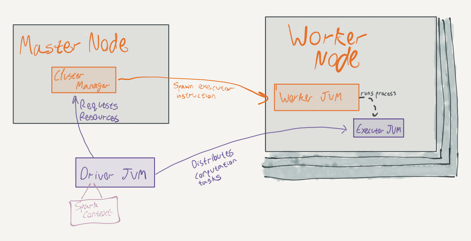
Here’s a diagram of a typical Spark application:

There are several moving pieces to that diagram. The master node and the worker nodes represent two physical machines. In our setup, they are represented by two containers. The master node runs the Cluster Manager JVM (also called the Spark Master), and the worker node runs the Worker JVM. These processes are independent of individual jobs running on the Spark cluster and typically outlive them.

The Driver JVM in the diagram represents the user code. In our case, the Spark REPL that we’ve launched is the driver. It is, in fact, a JVM that runs a Scala REPL with a preloaded sc: SparkContext object (and several other objects – we’ll see them in later posts in the series).

The SparkContext allows us to interact with Spark and load data into the cluster. It represents a session with the cluster manager. By opening such a session, the cluster manager will assign resources from the cluster’s available resources to our session and will cause the worker JVMs to spawn executors.

The data that we loaded (using sc.parallelize) was actually shipped to the executors; these JVMs actually do the heavy lifting for Spark applications. As the driver executes the user code, it distributes computation tasks to the executors. Before reading onwards, ask yourself: given Spark’s premise of parallel data processing, which parts of our snippet would it make sense to distribute?

Amusingly, in that snippet, there are exactly 5 characters of code that are directly running on the executors (3 if you don’t include whitespace!): _ + _ . The executors are only running the function closure passed to reduce.

To see this more clearly, let’s consider another snippet that does a different sort of computation:

In this snippet, which finds the Person with the maximum age out of those generated with age > 10, only the bodies of the functions passed to filter and reduce are executed on the executors. The rest of the program is executed on the driver.

As we’ve mentioned, the executors are also responsible for storing the data that the application is operating on. In Spark’s terminology, the executors store the RDD partitions – chunks of data that together comprise a single, logical dataset.

These partitions are the basic unit of parallelism in Spark; for example, the body of filter would execute, in parallel, on each partition (and consequently – on each executor). The unit of work in which a transformation is applied to a partition is called a Task. We will delve more deeply into tasks (and stages that are comprised of them) in the next post in the series.

Now that you know that executors store different parts of the dataset – is it really true that the function passed to reduce is only executed on the executors? In what way is reduce different, in terms of execution, from filter? Keep this in mind when we discuss actions and transformations in the next section.

RDD’s

Let’s discuss RDDs in further depth. As mentioned, RDDs represent a collection of data rows, divided into partitions and distributed across physical machines. RDDs can contain any data type (provided it is Serializable) – case classes, primitives, collection types, and so forth. This is a very powerful aspect as you can retain type safety whilst still distributing the dataset.

An important attribute of RDDs is that they are immutable: every transformation applied to them (such as map, filter, etc.) results in a new RDD. Here’s a short experiment to demonstrate this point; run this snippet, line-by-line, in the Spark shell:

The original RDD is unaffected by the filter operation – line 6 prints out 1000, while line 8 prints out a different count.

Another extremely important aspect to Spark’s RDDs is laziness. If you’ve run the previous snippet, you no doubt have noted that line 4 is executed instantaneously, while the lines that count the RDDs are slower to execute. This happens because Spark aggressively defers the actual execution of RDD transformations, until an action, such as count is executed.

To use more formal terms, RDDs represent a reified computation graph: every transformation applied to them is translated to a node in the graph representing how the RDD can be computed. The computation is promoted to a first-class data type. This presents some interesting optimization opportunities: consecutive transformations can be fused together, for example. We will see more of this in later posts in the series.

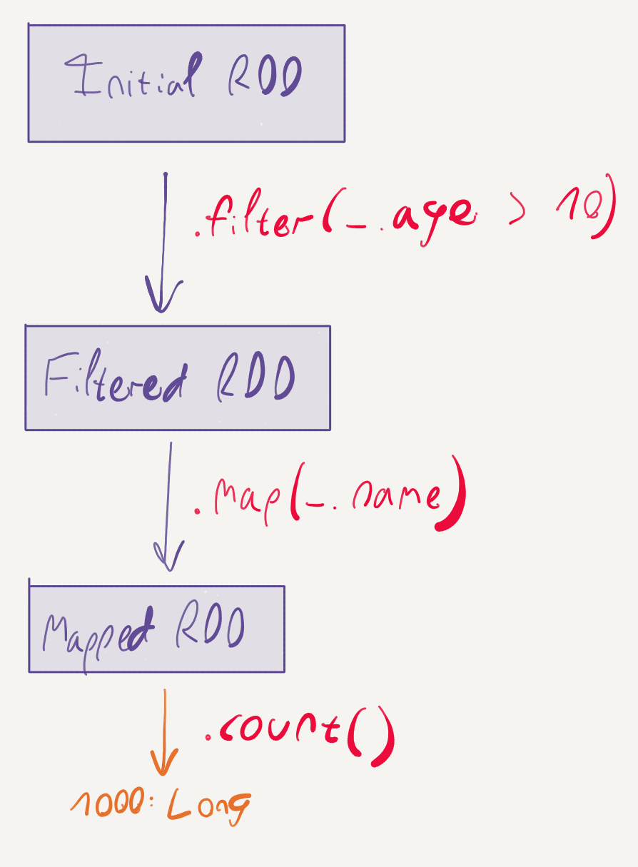
The difference between actions and transformations is important to keep in mind. As you chain transformations on RDDs, a chain of dependencies will form between the different RDDs being created. Only once an action is executed will the transformations run. This chain of dependencies is referred to as the RDD’s lineage.

A good rule of thumb for differentiating between actions and transformations in the RDD API is the return type; transformations often result in a new RDD, while actions often result in types that are not RDDs.

For example, the zipWithIndex method, with the signature:

def zipWithIndex(): RDD[(T, Long)]

is a transformation that will assign an index to each element in the RDD.

On the other hand, the take method, with the signature:

def take(n: Int): Array[T]

is an action; it results in an array of elements that is available in the driver’s memory space.

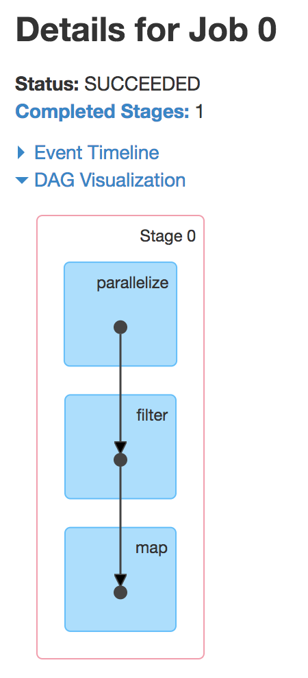
This RDD lineage is not just a logical concept; Spark’s internal representation of RDDs actually uses this direct, acyclic graph of dependencies. We can use this opportunity to introduce the Spark UI, available at http://localhost:4040/jobs/ after you launch the Spark shell. If you’ve run one of the snippets, You should see a table such as this:

By clicking the job’s description, you can drill down into the job’s execution and see the DAG created for executing this job:

The Spark UI can be extremely useful when diagnosing performance issues in Spark applications. We’ll expand more on it in later posts in the series.

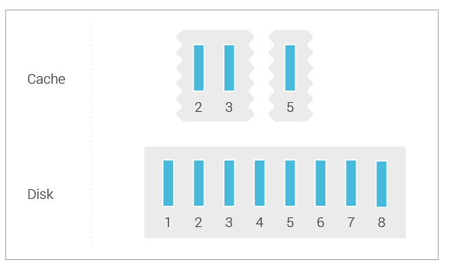
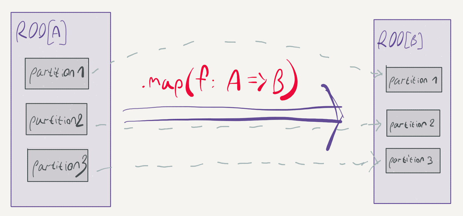
We can further divide transformations to narrow and wide transformations. To demonstrate the difference, consider what happens to the partitions of an RDD in a map:

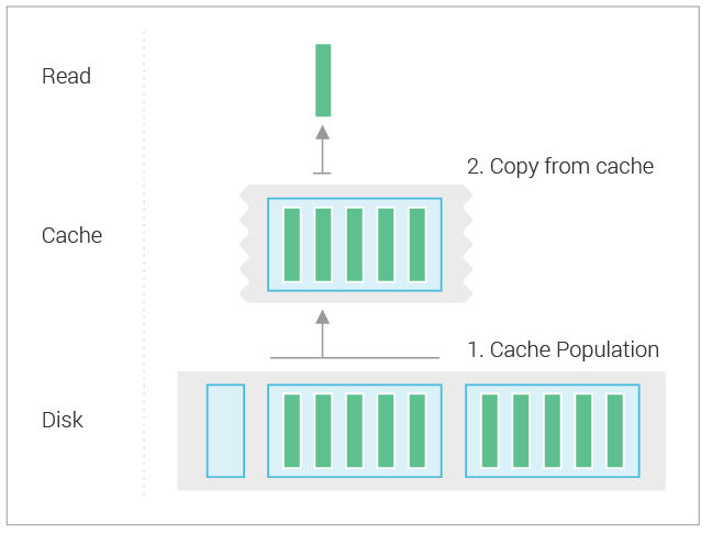
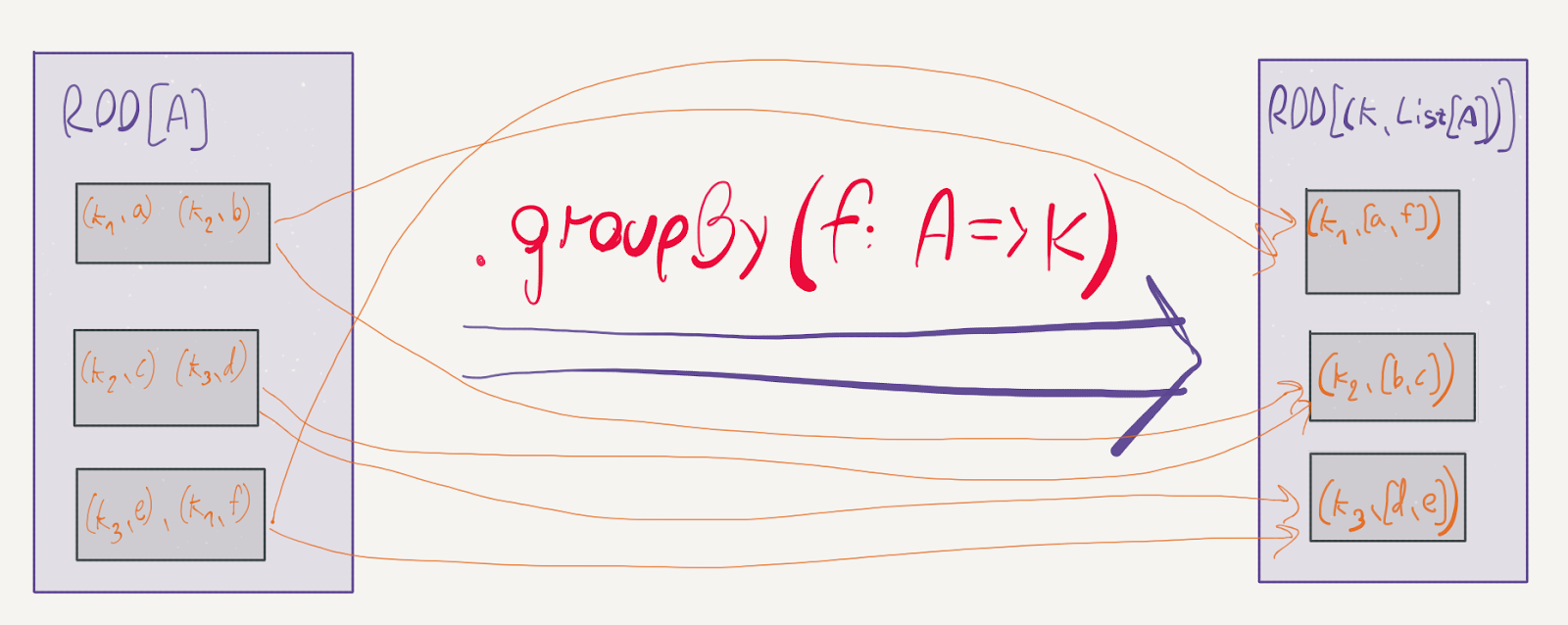
map is a prime example of a narrow transformation: the elements can stay in their respective partitions; there is no reason to move them around. Contrast this with the groupBy method:

def groupBy[K](f: T => K): RDD[(K, Iterable[T])]

As Spark executes the provided f for every element in the RDD, two elements in different partitions might be assigned the same key. This will cause Spark to shuffle the data in the partitions and move the two elements into the same physical machine in order to group them into the Iterable.

Avoiding data shuffles is critical for coaxing high performance out of Spark. Moving data between machines over the network in order to perform a computation is a magnitude slower than computing data within a partition.

Lastly, it is important to note that RDDs contain a pluggable strategy for assigning elements to partitions. This strategy is called a Partitioner and it can be applied to an RDD using the partitionBy method.

To summarize, RDDs are Spark’s representation of a logical dataset distributed across separate physical machines. RDDs are immutable, and every transformation applied to them results in a new RDD and a new entry in the lineage graph. The computations applied to RDDs are deferred until an action occurs.

We’re taking a bottom-up approach in this series to introducing Spark. RDDs are the basic building block of Spark’s APIs, and are, in fact, quite low-level for regular usage. In the next post, we will introduce Spark’s DataFrame and SQL APIs which provide a higher-level experience.

Scylla

Let’s move on to discuss Scylla. Scylla is an open-source NoSQL database designed to be a drop-in replacement for Apache Cassandra with superior performance. As such, it uses the same data model as Cassandra, supports Cassandra’s existing drivers, language bindings and connectors. In fact, Scylla is even compatible with Cassandra’s on-disk format.

This is where the similarities end, however; Scylla is designed for interoperability with the existing ecosystem, but is otherwise a ground-up redesign. For example, Scylla is written in C++ and is therefore free from nuisances such as stop-the-world pauses due to the JVM’s garbage collector. It also means you don’t have to spend time tuning that garbage collector (and we all know what black magic that is!).

Scylla’s Data Model

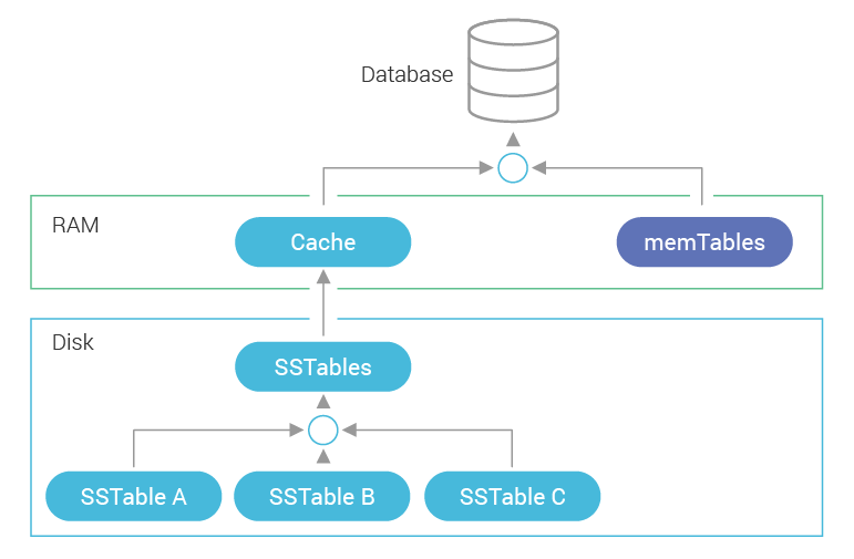
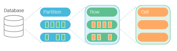
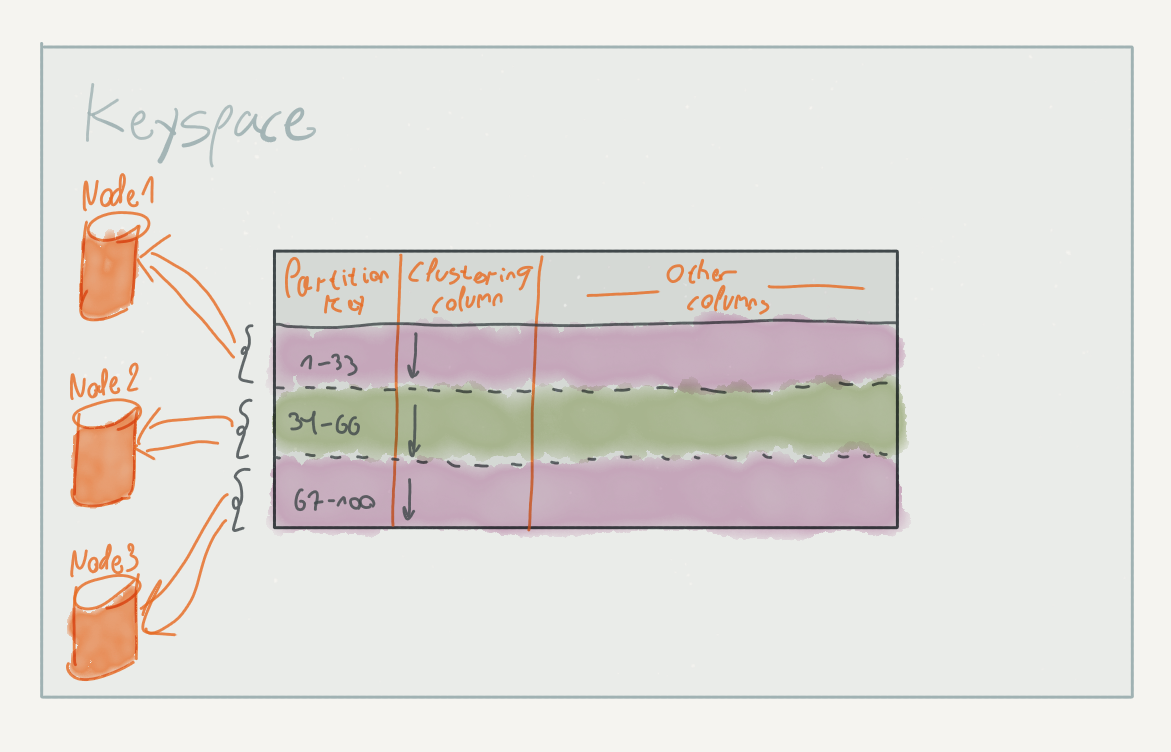
Scylla (and Cassandra) organize the stored data in tables (sometimes called column families in Cassandra literature). Tables contain rows of data, similar to a relational database. These rows, however, are divided up to partitions based on their partition key; within each partition, the rows are sorted according to their clustering columns.

The partition key and the clustering columns together define the table’s primary key. Scylla is particularly efficient when fetching rows using a primary key, as it can be used to find the specific partition and offset within the partition containing the requested rows.

Scylla also supports storing the usual set of data types in columns you would expect – integers, doubles, booleans, strings – and a few more exotic ones, such as UUIDs, IPs, collections and more. See the documentation for more details.

In contrast to relational databases, Scylla does not perform joins between tables. It instead offers rich data types that can be used to denormalize the data schema – lists, sets, and maps. These work best for small collections of items (that is, do not expect to store an entire table in a list!).

Moving upwards in the hierarchy, tables are organized in keyspaces– besides grouping tables together, keyspaces also define a replication strategy; see the documentation for CREATE KEYSPACE for more details.

Running Scylla Locally

To run Scylla locally for our experiments, we’ve added the following entry to our docker-compose.yaml file’s services section:

This will mount the ./data/node1 directory from the host machine’s current directory on /var/lib/scylla within the container, and limit Scylla’s resource usage to 1 processor and 256MB of memory. We’re being conservative here in order to run 3 nodes and make the setup interesting. Also, Spark’s much more of a memory hog, so we’re going easy on your computer.

NOTE: This setup is entirely unsuitable for a production environment. See ScyllaDB’s reference for best practices on running Scylla in Docker.

The docker-compose.yaml file provided in the sample repository contains 3 of these entries (with separate data volumes for each node), and to run the nodes, you can launch the stack:

After that is done, check on the nodes’ logs using docker-compose logs:

You should see similar log lines (among many other log lines!) on the other nodes.

There are two command-line tools at your disposal for interacting with Scylla: nodetool for administrative tasks, and cqlsh for applicative tasks. We’ll cover cqlsh and CQL in the next section. You can run both of them by executing them in the node containers.

For example, we can check the status of nodes in the cluster using nodetool status:

The output you see might be slightly different, but should be overall similar- you can see that the cluster consists of 3 nodes, their addresses, data on disk, and more. If all nodes show UN (*U*p, *N*ormal) as their status, the cluster is healthy and ready for work.

A Brief Overview of CQL

To interact with Scylla’s data model, we can use CQL and cqlsh – the CQL Shell. As you’ve probably guessed, CQL stands for Cassandra Query Language; it is syntactically similar to SQL, but adapted for use with Cassandra. Scylla supports the CQL 3.3.1 specification.

CQL contains data definition commands and data manipulation commands. Data definition commands are used for creating and modifying keyspaces and tables, while data manipulation commands can be used to query and modify the tables’ contents.

For our running example, we will use cqlsh to create a table for storing stock price data and a keyspace for storing that table. As a first step, let’s launch it in the node container:

We can use the DESC command to see the existing keyspaces:

The USE command will change the current keyspace; after we apply it, we can use DESC again to list the tables in the keyspace:

These are useful for exploring the currently available tables and keyspaces. If you’re wondering about the available commands, there’s always the HELP command available.

In any case, let’s create a keyspace for our stock data table:

As we’ve mentioned before, keyspaces define the replication strategy for the tables within them, and indeed in this command we are defining the replication strategy to use SimpleStrategy. This strategy is suitable for use with a single datacenter. The replication_factor setting determines how many copies of the data in the keyspace are kept; 1 copy means no redundancy.

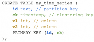
With the keyspace created, we can create our table:

Our table will contain a row per symbol, per day. The query patterns for this table will most likely be driven by date ranges. Within those date ranges, we might be querying for all symbols, or for specific ones. It is unlikely that we will drive queries on other columns.

Therefore, we compose the primary key of symbol and day. This means that data rows will be partitioned between nodes according to their symbol, and sorted within the nodes by their day value.

We can insert some data into the table using the following INSERT statement:

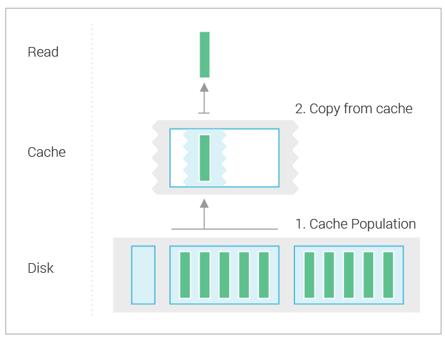
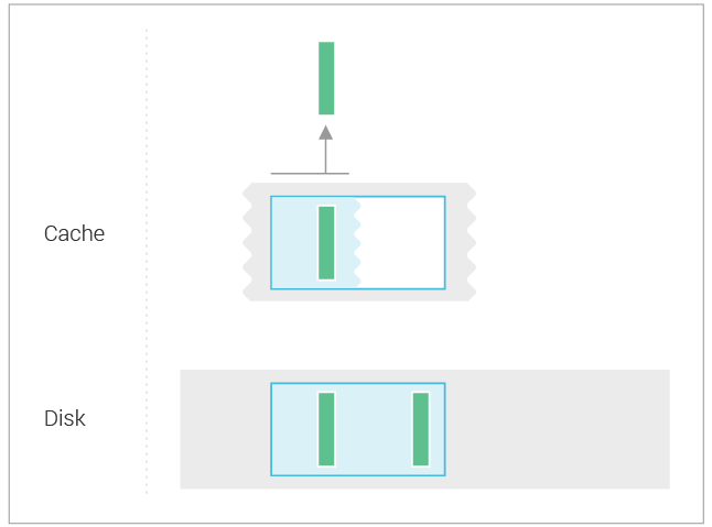
Now, let’s consider the following query under that data model – the average close price for all symbols in January 2010:

This would be executed as illustrated in the following diagram:

Note that the partitioning structure allows for parallel reduction of the data in each partition when computing the average. The sum of all closing prices is computed in each partition, along with the count of rows in each partition. These sum and count pairs can then be reduced between the partitions.

If this reminds you of how RDDs execute data processing tasks – it should! Partitioning data by an attribute between several partitions and operating on the partitions in parallel is a very effective way of handling large datasets. In this series, we will show how you can efficiently copy a Scylla partition into a Spark partition, in order to continue processing the data in Spark.

With the data in place, we can finally move on to processing the data stored in Scylla using Spark.

The Datastax Spark/Cassandra Connector

The Datastax Spark/Cassandra connector is an open-source project that will allow us to import data in Cassandra into Spark RDDs, and write Spark RDDs back to Cassandra tables. It also supports Spark’s SQL and DataFrame APIs, which we will discuss in the next post.

Since Scylla is compatible with Cassandra’s protocol, we can seamlessly use the connector with it.

We’ll need to make sure the connector ends up on the Spark REPL’s classpath and configure it with Scylla’s hostname, so we’ll re-launch the shell in the Spark master’s container, with the addition of the --packages and --conf arguments:

The shell should now download the required dependencies and make them available on the classpath. After the shell’s prompt shows up, test that everything worked correctly by making the required imports, loading the table as an RDD and running .count() on the RDD:

The call to count should result in 4 (or more, if you’ve inserted more data than listed in the example!).

The imports that we’ve added bring in syntax enrichments to the standard Spark data types, making the interaction with Scylla more ergonomic. You’ve already seen one of those enrichments: sc.cassandraTable is a method added to SparkContext for conveniently creating a specialized RDD backed by a Scylla table.

The type of that specialized RDD is CassandraTableScanRDD[CassandraRow]. As hinted by the type, it represents a scan of the underlying table. The connector exposes other types of RDDs; we’ll discuss them in the next post.

Under the hood, the call to .count() translates to the following query in Scylla:

The entire table is loaded into the Spark executors, and the rows are counted afterward by Spark. If this seems inefficient to you – it is! You can also use the .cassandraCount() method on the RDD, which will execute the count directly on Scylla.

The element contained in the RDD is of type CassandraRow. This is a wrapper class for a sequence of untyped data, with convenience getters for retrieving fields by name and casting to the required type.

Here’s a short example of interacting with those rows:

This will extract the first row from the RDD, and extract the symbol and the close fields’ values. Note that if we try to cast the value to a wrong type, we get an exception:

Again, as in the case of row counting, the call to first will first load the entire table into the Spark executors, and only then return the first row. To solve this inefficiency, the CassandraRDD class exposes several functions that allow finer-grained control over the queries executed.

We’ve already seen cassandraCount, that delegates the work of counting to Scylla. Similarly, we have the where method, that allows you to specify a CQL predicate to be appended to the query:

The benefit of the where method compared to applying a filter transformation on an RDD can be drastic. In the case of the filter transformation, the Spark executors must read the entire table from Scylla, whereas when using where, only the matching data will be read. Compare the two queries that’ll be generated:

Obviously, the first query is much more efficient!

Two more useful examples are select and limit. With select, you may specify exactly what data needs to be fetched from Scylla, and limit will only fetch the specified number of rows:

The query generated by this example would be as follows:

These methods can be particularly beneficial when working with large amounts of data; it is much more efficient to fetch a small subset of data from Scylla, rather than project or limit it after the entire table has been fetched into the Spark executors.

Now, these operations should be enough for you to implement useful analytical workloads using Spark over data stored in Scylla. However, working with CassandraRow is not very idiomatic to Scala code; we’d much prefer to define data types as case classes and work with them.

For that purpose, the connector also supports converting the CassandraRow to a case class, provided the table contains columns with names matching the case class fields. To do so, we specify the required type when defining the RDD:

The connector will also helpfully translate columns written in snake case (e.g., first_name) to camel case, which means that you can name both your table columns and case class fields idiomatically.

Summary

This post has been an overview of Spark, Scylla, their architectures and the Spark/Cassandra connector. We’ve taken a broad-yet-shallow look at every component in an attempt to paint the overall picture. Over the next posts, we will dive into more specific topics. Stay tuned!

Next Steps

  • Scylla Summit 2018 is around the corner. Register now!
  • Learn more about Scylla from our product page.
  • See what our users are saying about Scylla.
  • Download Scylla. Check out our download page to run Scylla on AWS, install it locally in a Virtual Machine, or run it in Docker.
  • Take Scylla for a Test drive. Our Test Drive lets you quickly spin-up a running cluster of Scylla so you can see for yourself how it performs.

The post Hooking up Spark and Scylla: Part 1 appeared first on ScyllaDB.


AdGear and ScyllaDB at the Big Data Montreal Meetup

$
0
0

AdGear and ScyllaDB

Last month, Mina Naguib, Director of Operations Engineering at AdGear, and Glauber Costa, VP of Field Engineering at ScyllaDB, teamed up at the Big Data Montreal meetup to discuss Real-time Big Data at Scale, examining how Scylla helped Adwords achieve their goal of 1 million queries per second with single-digit millisecond latencies.

Click the video below to see AdGear present their real-time advertising use case along with the results of switching from Cassandra to Scylla. Glauber explains how Scylla enabled AdGear to achieve high throughput at predictably low latencies, all while keeping TCOs under tight control.

AdGear is an online ad serving platform that compiles vast amounts of consumer data that’s used by online exchanges to bid on ad placements in real-time. AdGear has very little time to enter a bid; auctions often close in less than 100 milliseconds. Cassandra simply couldn’t keep up. While it performed about 1,000,000 bids per second, the latency and tuning complexity made it costly and difficult to keep up with online exchanges.

In this talk, Mina discusses how Scylla enables AdGear to hit their extreme throughput requirements, serving the same number of requests as Cassandra with half the hardware. Originally running a 31-node Cassandra cluster, AdGear easily downsized to a 16-node Scylla cluster in which each node serves more than twice as many queries as Cassandra’s. At peak traffic, read latency fell from 21 milliseconds to less than 5 ms on Scylla.

Glauber picks up and discusses common and familiar problems with Cassandra; unpredictable latency, tuning complexity, node sprawl, and garbage collection woes. As Glauber shows, Scylla users can accomplish more with less hardware, demonstrating that a single Scylla node can achieve 1 million OPS, with 1 ms 99% latency, all while auto-tuning and scaling up and out efficiently and painlessly.

To learn more about Scylla’s close-to-the-hardware architecture and how it helped AdGear amp up their ad serving platform, check out the video above.

Next Steps

  • Scylla Summit 2018 is around the corner. Register now!
  • Learn more about Scylla from our product page.
  • See what our users are saying about Scylla.
  • Download Scylla. Check out our download page to run Scylla on AWS, install it locally in a Virtual Machine, or run it in Docker.
  • Take Scylla for a Test drive. Our Test Drive lets you quickly spin-up a running cluster of Scylla so you can see for yourself how it performs.

The post AdGear and ScyllaDB at the Big Data Montreal Meetup appeared first on ScyllaDB.

The Mutant Monitoring System Scylla Training Series

$
0
0

At ScyllaDB, we created our Mutant Monitoring System blog series as a fun and informative way to teach users the ropes. As a quick recap of the backstory, mutants have emerged from the shadows and are now wreaking havoc on the earth. Increased levels of malicious mutant behavior pose a threat to national security and the general public. To better protect the citizens and understand more about the mutants, the Government enacted the Mutant Registration Act. As required by the act, each mutant must wear a small device that reports on his/her actions every second. The overall mission is to help the Government keep the Mutants under control by building a Mutant Monitoring System (MMS).

The Mutant Monitoring series has been a great tool used to train new and experienced Scylla users on key concepts such as setup, failover, compactions, multi-datacenters, and integrations with third-party applications. The series is also good for developers to learn how to use Scylla in their applications in various programming languages.

In this post, I will go over each day of our training series and explain what you can get out of it.

Day 1: Setting up Scylla. On the first day, we explored the backstory of Division 3 and decided that Scylla is the best choice for the database backend. Using Docker, we set up a Scylla cluster and created the initial mutant catalog keyspace and table. After the tables were made, we added a few mutants to the catalog that serve as our main mutant characters for the entire series.

Day 2: Building the Tracking System. For day two, we picked up where we left off and built the tracking system which is a time-series collection of mutant data such as timestamp, location, and attributes based on their abilities. We also discussed the schema design in depth and went over the compaction strategy and clustering key and how to insert data and run queries.

Day 3: Analyzing Data. With the tracking system setup, we were now able to begin analyzing the data in day 3 and did this using Presto in Docker. Presto is a distributed SQL query engine for Big Data technologies like Scylla. With it, we showed how to run complex queries such as full-text search, comparing values, and querying data.

Day 4: Node Failure Scenarios. At Division 3, our mutant data-centers were experiencing more and more cyber attacks by evil mutants and sometimes we experienced downtime and cannot track our IoT sensors. By day 4, we realized that we needed to prepare for disaster scenarios so that we know for sure that we can survive an attack. In this exercise, we went through a node failure scenario, consistency levels, and how to add a node and repair the Scylla cluster.

Day 5: Visualizing Data with Apache Zeppelin. On day 5, we learned how to use Apache Zeppelin to visualize data from the Mutant Monitoring System. Apache Zeppelin is a Java Web-based solution that allows users to interact with a variety of data sources like MySQL, Spark, Hadoop, and Scylla. Once in Zeppelin, you can run CQL queries and view the output in a table format with the ability to save the results. Also, the query can be visualized in an array of different graphs.

Day 6 and 7: Multi-datacenter Scylla Deployment. Division 3 decided that they must prepare for disaster readiness by expanding the Scylla cluster across geographic regions in a multi-datacenter configuration. On day 6, we will set up a new Scylla cluster in another datacenter and learned how to convert our existing keyspaces to be stored in both datacenters and went over site failure scenarios. On day 7, we expanded this topic and went over consistency levels for multi-datacenter Scylla deployments.

Day 8: Scylla Monitoring. For day 8, we explained how to set up the Scylla Monitoring Stack which runs in Docker and consists of Prometheus and Grafana containers. We chose to run the monitoring stack so we can examine important Scylla specific details such as performance, latency, node availability, and more from the cluster.

Day 9: Connecting to Scylla with Node.js. Division 3 wanted to teach their development team how to create applications that can interact with the Scylla Cluster so they can build the next-generation tools for the Mutant Monitoring System. On day 9, we explored how to connect to a Scylla cluster using Node.js with the Cassandra driver and also went over the available Cassandra API’s for other programming languages.

Day 10: Backup and Restore. On day 10 we were told that Division 3 implemented a new policy for Scylla Administrators to learn how to backup and restore the mutant data in the cluster. Throughout the lesson, we explained how to simulate data loss and how to backup and restore data from Scylla.

Days 11 and 12: Using the Cassandra Java Driver. Division 3 decided that we must use more applications to connect to the mutant catalog and decided to hire Java developers to create powerful applications that can monitor the mutants. On day 11 and 12, we will explore how to connect to a Scylla cluster using the Cassandra driver for Java using basic query statements and then explained how to modify a Java program to use prepared statements

Day 13: Materialized Views. The Mutant Monitoring System had been receiving a lot of data and Division 3 wanted to find better ways to sort and store data so it can be quickly analyzed with applications. Luckily, having found an exciting feature in Scylla called Materialized Views, they provided us with directives to learn how to use it to help our application developers prevent further acts of terror. On day 13, we explained what Materialized Views are and how to use it with the Mutant Monitoring System.

Day 14: Using Apache Spark with Scylla. On day 14, Division 3 wanted to dive back into data analytics to learn how to prevent the attacks. For this training, we went over how to use Apache Spark, Hive, and Superset to analyze and visualize the data from the Mutant Monitoring system.

Day 15: Storing Binary Blobs in Scylla. Day 15 concluded our final Java programming series by explaining how to store binary files in Scylla. With this ability, we were able to learn how to store images of the mutants in the catalog keyspace using the blob table type. With the images stored, Division 3 was able to see what the mutant looks like whenever they want.

Day 16: The Mutant Monitoring Web Console. Day 16 is the final post in the series for now and we explained how to create a Mutant Monitoring Web Console in Node.js. The web console has a central interface that displays photos of the mutants and their basic information, as well as tracking information such as heat, telepathy, speed, and current location.

We hope that the Mutant Monitoring System has been educational for Scylla users. Throughout this series, we discussed a variety of topics ranging from running and configuring Scylla, recovering from disasters, expanding across multiple datacenters, using Scylla with different programming languages, and how to integrate Scylla with third-party applications like Spark and Presto. This series is done for now but we hope that the practical knowledge it provides will live on for some time.

Next Steps

  • Scylla Summit 2018 is around the corner. Register now!
  • Learn more about Scylla from our product page.
  • See what our users are saying about Scylla.
  • Download Scylla. Check out our download page to run Scylla on AWS, install it locally in a Virtual Machine, or run it in Docker.
  • Take Scylla for a Test drive. Our Test Drive lets you quickly spin-up a running cluster of Scylla so you can see for yourself how it performs.

The post The Mutant Monitoring System Scylla Training Series appeared first on ScyllaDB.

The Cost of Containerization for Your Scylla

$
0
0

 Cost Containerization


The ubiquity of Docker as a packaging and deployment platform is ever growing. Using Docker containers relieves the database operator from installing, configuring, and maintaining different orchestration tools. In addition, it standardizes the database on a single orchestration scheme that is portable across different compute platforms.

There is, however, a performance payoff for the operational convenience of using containers. This is to be expected because of the extra layer of abstraction (the container itself), relaxation on resource isolation, and increased context switches. This solution is known to be computationally costly, which is exacerbated on a shard-per-core architecture such as Scylla. This article will shed light on the performance penalties involved in running Scylla on Docker, where the penalties are coming from, and the tuning steps Docker users can take to mitigate them. In the end, we demonstrate that it is possible to run Scylla on Docker containers by paying no more than a 3% performance penalty in comparison with the underlying platform.

Testing Methodology

The initial testing used an Amazon Web Service i3.8xlarge instance as a baseline for performance. Once the baseline performance was established, we used the same workload on a Docker base deployment container and compared the results.

Testing included:

  • Max throughput for write workloads
  • Latency comparisons at targeted read workload

The hardware and software setup used for testing are described in Appendix B
The different workloads are described in Appendix C.

We tested the same workload in four different configurations:

  • AMI: Scylla 2.2 AMI, running natively on AWS without any further tuning
  • Docker default: Scylla 2.2 official Dockerhub image without any further tuning
  • --cpuset: Scylla 2.2 Dockerhub image, but with CPU pinning and isolation of network interrupts to particular cores, mimicking what is done in the Scylla AMI.
  • --network host: Aside from the steps described in –cpuset, also bypassing the Docker virtualized networking by using the host network.

Max Throughput Tests

We chose a heavy disk I/O workload in order to emulate a cost-effective, common scenario. Max write throughput tests were obtained using the normal distribution of partition, in which the median is the half of the populated range and standard deviation is one-third of the median. The results are shown in Figure 1.

Figure 1: Maximum throughput comparison between a Scylla 2.2 AMI running on an AWS i3.8xlarge (blue), and various Docker configurations. With the default parameters meant to run in shared environments, there is a 69% reduction in peak throughput. However, as we optimize, the difference can be reduced to only  3%.

Scylla in a Docker container showed 69% reduction on write throughput using our default Docker image. While some performance reduction is expected, this gap is significant and much bigger than one would expect. We attribute it to the fact that none of the close-to-the-hardware optimizations usually employed by Scylla are present. The results get closer to the underlying platform’s performance when Scylla controlled the resources and allocated the needed tasks to the designated CPU, IO channel, and network port. A significant portion of the performance was recovered (11% reduction) with CPU Pinning and perftune.py (to tune the NIC and disks in the host) script execution. Going even further, using the host network and removing the Docker network virtualization using the --network host parameter brought us to a 3% reduction on overall throughput. One of the strong Docker features is the ability to separate networking traffic coming to each Docker instance on the same machine (as described here). If one uses the --network host parameter,  he/she will no longer be able to do that since Docker is going to hook up to the host networking stack directly.

Latency Test Results

To achieve the best latency results, we issued a read workload to the cluster at a fixed throughput. The throughput is the same for all cases to make the latency comparison clear. We executed the tests on the wide range of the populated data set for 1 hour, making sure that the results are coming from both cache and disk. The results are shown in Figure 2.

Figure 2: 99.9th, 99th, 95th and average latency for a read workload with fixed throughput with the Scylla 2.3 AMI, in blue, and with the various Docker configurations. There is a stark increase in the higher percentiles with the default configuration where all optimizations are disabled. But as we enabled them the difference essentially disappears.

While the difference in percentage (up to 40%) might be significant from the AMI to the Docker image, the numerical difference is in the single digit millisecond. But after network and CPU pinning and removing the Docker network virtualization layer, the differences become negligible. For users who are extremely latency sensitive, we still recommend using a direct installation of Scylla. For users looking to benefit from the ease of Docker usage, the latency penalty is minimal.

Analysis

We saw in the results of the previous runs that users who enable specific optimizations can achieve with Docker setups performance levels very close to what they would in the underlying platform. But where is the difference coming from?

The first step is obvious: Scylla employs a polling thread-per-core architecture, and by pinning shards to the physical CPUs and isolating network interrupts the number of context switches and interrupts is reduced.

As we saw, once all CPUs are pinned we can achieve throughput that is just 11% worse than our underlying platform. It is enlightening at this point to look at Flamegraphs for both executions. They are presented in Figures 3 and 4 below:

Figure 3: Flamegraphs obtained during a max-throughput write workload with the Scylla 2.2 AMI.

Figure 4: Flamegraphs obtained during the same workload against Scylla running in Docker containers with its CPUs pinned and interrupts isolated.

As expected, the Scylla part of the execution doesn’t change much. But to the left of the Flamegraph we can see a fairly deep callchain that is mostly comprised of operating system functions. As we zoom into it, as shown in Figures 5 and 6, we can see that those are mostly functions involved in networking. Docker virtualizes the network as seen by the container. Therefore, removing this layer can bring back some of the performance as we saw in Figures 1 and 2.


Figure 5: Zooming in to the Flamegraphs. The Scylla 2.2 AMI.

Figure 6: Scylla running on Docker with all CPUs pinned and network interrupts isolated.

Where Does the Remaining Difference Come From?

After all of the optimizations were applied, we still see that Docker is 3% slower than the underlying platform. Although this is acceptable for most deployments, we would still like to understand why. Hints as to why can be seen in the very Flamegraphs in Figures 3-6. We see calls to seccomp that are present in the Docker setup but not in the underlying platform. We also know for a fact that Docker containers are executed within Linux cgroups, which are expected to add overhead.

We disabled security profiles by using the --security-opt seccomp :unconfined Docker parameter. Also, it is possible to manually move tasks out of cgroups by using the cgdelete utility. Executing the peak throughput tests again, we now see no difference in throughput between Docker and the underlying platform. Understanding where the difference comes from adds educational value. However, as we consider those to be essential building blocks of a sane Docker deployment, we don’t expect users to run with those disabled.

Conclusion

Containerizing applications is not free. In particular, processes comprising the containers have to be run in Linux cgroups and the container receives a virtualized view of the network. Still, the biggest cost of running a close-to-hardware, thread-per-core application like Scylla inside a Docker container comes from the opportunity cost of having to disable most of the performance optimizations that the database employs in VM and bare-metal environments to enable it to run in potentially shared and overcommitted platforms.

The best results with Docker are obtained when resources are statically partitioned and we can bring back bare-metal optimizations like CPU pinning and interrupt isolation. There is only a 10% performance penalty in this case as compared to the underlying platform – a penalty that is mostly attributed to the network virtualization. Docker allows users to expose the host network directly for specialized deployments. In cases in which this is possible, we saw that the performance difference compared to the underlying platform falls down to 3%.

Appendix A: Ways to Improve Performance in a Containerized Environment

As we demonstrated in previous articles like An Overview of Scylla Architecture and its underlying framework Seastar, Scylla uses a shared-nothing approach and pins each Scylla shard to a single available CPU.

Scylla already provides some guidelines on how to improve Scylla performance on Docker. Here we present a practical example on an i3.8xlarge AWS instance and showcase how to use network IRQ and CPU pinning.

Network Interrupts

Scylla checks the available network queues and available CPUs during the setup. If there are not enough queues to distribute network interrupts across all of the cores, Scylla will isolate some CPUs for this purpose. Also, if irqbalance is installed it will add the CPUs dedicated to networking to the list of irqbalance banned CPUs. For that Scylla uses the perftune script, distributed with Scylla packages. It is still possible to run the same script in the host in preparation for running Docker containers. One caveat is that those changes are not persisted and have to be applied every time the machine is restarted.

In the particular case of i3.8xlarge perftune will isolate CPUs 0 and 16 for the sole purpose of handling network interrupts:

For proper isolation, the CPUs handling network interrupts shouldn’t handle any database load. We can use a combination of perftune.py and hex2list.py to discover exactly what are the CPUs that are free of network interrupts:

Shard-per-core Architecture and CPU Pinning

When we use Scylla inside a container, Scylla is unaware of the underlying CPUs in the host. As a result, we can see drastic performance impact (50%-70%) due to context switches, hardware interrupts, and the fact that Scylla needs to stop employing polling mode. In order to overcome this limitation, we recommend users to statically partition the CPU resources to b assigned to the container and letting the container take full control of its shares. This can be done using the --cpuset option. In this example, we are using an i3.8xlarge (32 vcpus) and want to run a single container in the entire VM. We will pass --cpuset 1,15-17-31 ensuring that we pin 30 shards to 30 vCPUs. The two remaining vCPUs will be used for network interrupts as we saw previously. It is still possible to do this when more than one container is present in the box, by partitioning accordingly.

Appendix B: Setup and Systems Used for Testing (AWS)

Hardware

Throughput tests
1 x i3.8xlarge (32 CPUs 244GB RAM 4 x 1900GB NVMe 10 Gigabit network card) Scylla node
2 x c4.8xlarge (36 CPUs 60GB RAM 10 Gigabit network card) writers running 4 cassandra-stress instance each.

Latency tests
1 x i3.8xlarge (32 CPUs 244GB RAM 4 x 1900GB NVMe 10 Gigabit network card) Scylla node
2 x c4.8xlarge (36 CPUs 60GB RAM 10 Gigabit network card) readers running 4 cassandra-stress instance each.

Software

Scylla 2.2 AMI (ami-92dc8aea region us-west-2 [Oregon])
Docker version 1.13.1, build 94f4240/1.13.1
Perftune.py from scylla-tools

Provisioning Procedure

AMI
AMI deployed using AWS Automation

Docker

Docker --cpuset

Docker --network host

Appendix C: Workloads

Dataset

5 Columns, 64 bytes per column, 1500000000 partitions. Total Data: ~480GB
2 Loaders running 1 cassandra-stress, 750000000 interactions each
cassandra-stress commands:

Loader 1:

Loader 2:

Write Max Throughput Test

2 Loaders running 4 cassandra-stress each for 1 hour.
cassandra-stress commands:

Loader 1:

Loader 2:

30K IOPs Read Latency Test

2 Loaders running 4 cassandra-stress each for 1 hour.
cassandra-stress commands:

Loader 1:

Loader 2:

The post The Cost of Containerization for Your Scylla appeared first on ScyllaDB.

Upcoming Improvements to Scylla Streaming Performance

$
0
0

Scylla Streaming

Streaming in Scylla is an internal operation that moves data from node to node over a network. It is the foundation of various Scylla cluster operations. For example, it is used by an “add node” operation to copy data to a new node in a cluster. It is also used by a “decommission” operation that removes a node from a cluster and streams the data it holds to the other nodes. Another example is a “rebuild” operation that rebuilds the data that a node should hold from replicas on other nodes. It is also used by a “repair” operation that is used to synchronize data between nodes.

In this blog post, we will take a closer look at how Scylla streaming works in detail and how the upcoming Scylla 2.4’s new streaming improves streaming bandwidth by 240% and reduces the time it takes to perform a “rebuild” operation by 70%.

How Scylla Streaming Works

The idea behind Scylla streaming is very simple. It’s all about reading data on one node, sending it to another node, and applying the data to disk. The diagram below shows the current path of data streaming. The sender creates sstable readers to read the rows from sstables on disk and sends them over the network. The receiver receives the rows from the network and writes them to the memtable. The rows in memtable are flushed into sstables periodically or when the memtable is full.

How We’re Improving Scylla Streaming

You can see that on the receiver side, the data is applied to a memtable. In normal CQL writes, memtables help by sorting the CQL writes in the form of mutations. When the CQL writes in memtables are flushed to an SSTable, the mutations are sorted. However, when streaming, the mutations are already sorted. This is because they are in the same order when the sender reads the mutations from the SSTable. That’s great! We can remove the memtable from the process. The advantages are:

  • Less memory consumption. The saved memory can be used to handle your CQL workload instead.
  • Less CPU consumption. No CPU cycles are used to insert and sort memtables.
  • Bigger SSTables and fewer compactions. Once the Memtable is full, it is flushed to an SSTable on disk. This happens during the whole streaming process repeatedly, thus generating many smaller SSTable files. This volume of SSTables adds pressure to compaction. By removing the memtable from the streaming process, we can write the mutations to a single SSTable.

If we look at the sender and receiver as a sandwich, the secret sauce is the Seastar RPC framework. To send a row, a Seastar RPC call is invoked. The sender invokes the RPC call repetitively until all the rows are sent. The RPC call is used in request-response models. For streaming, the goal is to send a stream of data with higher throughput and less time and not to request the remote node to process the data and give a response with lower latency for each individual request. Thus, it makes more sense to use the newly introduced Seastar RPC Streaming interface. With the new Seastar RPC Streaming interface, we need to use the RPC call only once to get handlers called Sink and Source, dramatically reducing the number of RPC calls to send streaming data. On the sender side, the rows are pushed to the Sink handler, which sends them over the network. On the receiver side, the rows are pulled from the Source handler. It’s also worth noting that we can remove the batching at the streaming layer since the Seastar RPC streaming interface will do the batching automatically.

With the new workflow in place, the new streaming data path looks like this:

Performance Improvements

In this part, we will run tests to evaluate the streaming performance improvements. For this, we chose to use the rebuild operation that streams data from existing nodes to rebuild the database. Of course, the rebuild operation uses Scylla streaming.

We created a cluster of 3 Scylla nodes on AWS using i3.xlarge instance. (You can find the setup details at the end of this blog post.) Afterward, we created a keyspace with a replication factor of 3 and inserted 1 billion partitions to each of the 3 nodes. After the insertion, each node held 240 GiB of data. Lastly, we removed all the SSTables on one of the nodes and ran the “nodetool rebuild” operation. The sender nodes with the replicas send the data to the receiver node in parallel. Thus, in our test, there were two nodes streaming in parallel to the node that ran the rebuild operation.

We compared the time it took to complete the rebuild operation and the streaming bandwidth on the receiver node before and after the new streaming changes.

Tests Old Scylla Streaming New Scylla Streaming Improvement
Time To Rebuild 170 minutes 50 minutes 70%
Streaming Bandwidth 36 MiB/s 123 MiB/s 240%

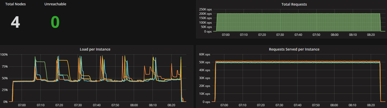
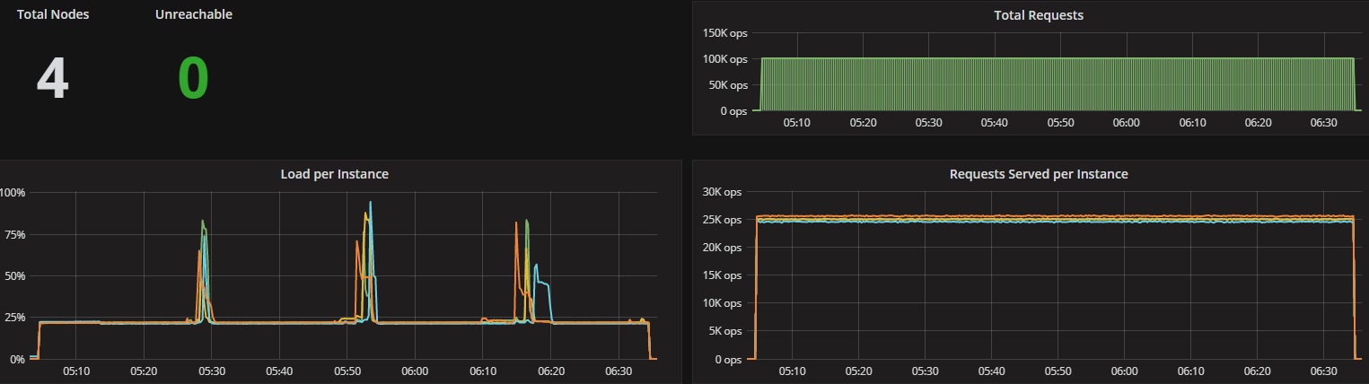
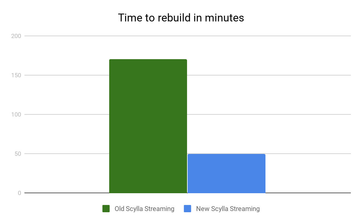
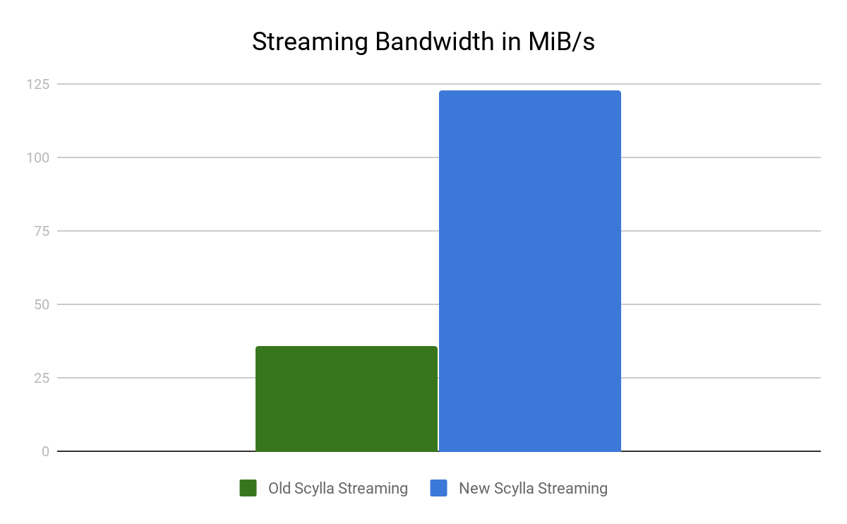
To look at the streaming performance on bigger machines, we did the above test again with 3 i3.8xlarge nodes. Since the instance is 8 times larger, we inserted 8 billion partitions to each of the 3 nodes. Each node held 1.89TiB of data. The test results are in the tables below.

Tests Old Scylla Streaming New Scylla Streaming Improvement
Time To Rebuild 218 minutes 66 minutes 70%
Streaming Bandwidth 228 MiB/s 765 MiB/s 235%

Conclusion

With our new Scylla streaming, streaming data is written to the SSTable on disk directly and skips the memtable completely resulting in less memory and CPU usage and less compaction. The data is sent over network utilizing the new Seastar RPC Streaming interface.

The changes described here will be released in the upcoming Scylla 2.4 release. It will make the Scylla cluster operations like add new node, decommission node and repair node even faster.
You can follow our progress at implementing the streaming improvement on GitHub: #3591.

Next Steps

  • Scylla Summit 2018 is around the corner. Register now!
  • Learn more about Scylla from our product page.
  • See what our users are saying about Scylla.
  • Download Scylla. Check out our download page to run Scylla on AWS, install it locally in a Virtual Machine, or run it in Docker.
  • Take Scylla for a Test drive. Our Test Drive lets you quickly spin-up a running cluster of Scylla so you can see for yourself how it performs.

Setup Details

DB Nodes: 3
Instance Type: i3.xlarge / i3.8xlarge
Replication Factor (RF): 3
Consistency Level (CL): QUORUM
Compaction Strategy: Size-Tiered
Scylla Version: Scylla master commit 31d4d37161bdc26ff6089ca4052408576a4e6ae7 with the new streaming disabled / enabled.

The post Upcoming Improvements to Scylla Streaming Performance appeared first on ScyllaDB.

Upcoming Enhancements to Scylla’s Filtering Implementation

$
0
0

Filtering Implementation


The upcoming Scylla 2.4 release will come with enhanced filtering support. One of the reasons we’re making this enhancement is due to the Spark-Cassandra connector’s reliance on ALLOW FILTERING support when generating CQL queries. The first part of this post provides a quick overview of what filtering is and why it can be useful. Then we will discuss why it can hurt performance and recommended alternatives. Finally, we’ll cover the caveats of Scylla’s filtering implementation.

ALLOW FILTERING Keyword

Queries that may potentially hurt a Scylla cluster’s performance are, by default, not allowed to be executed. These queries include those that restrict:

  • Non-key fields (e.g. WHERE v = 1)
  • Parts of primary keys that are not a prefixes (e.g. WHERE pk = 1 and c2 = 3)
  • Partition keys with something else other than an equality relation (e.g. WHERE pk >= 1)
  • Clustering keys with a range restriction and then by other conditions (e.g. WHERE pk =1 and c1 > 2 and c2 = 3)

Scylla is expected to be compatible with Cassandra in qualifying queries for filtering.

ALLOW FILTERING is a CQL keyword that can override this rule, but for performance reasons, please use it with caution. Let’s take a look at an example scenario – a database designed for a restaurant that wants to keep all of their menu entries in one place.

You can use the following code snippets to build a sample restaurant menu. This example will serve as a reference in the proceeding sections.

Now, with the test table initialized, let’s see which SELECT statements are potential filtering candidates. Queries based on primary key prefixes will work fine and filtering is not needed:

SELECT * FROM menu WHERE category = 'starters' and position = 3;

SELECT * FROM menu WHERE category = 'soups';

Now let’s take a look at queries below.

For an affordable meal:

SELECT * FROM menu WHERE price <= 10. ALLOW FILTERING;

For one specific dish:

SELECT * FROM menu WHERE name = 'sour rye soup' ALLOW FILTERING;

For all dishes that are listed first, but with a very specific price:

SELECT * FROM menu WHERE position = 1 and price = 10.5 ALLOW FILTERING;

For cheap starters:

SELECT * FROM menu WHERE category = 'starters' and price <= 10 ALLOW FILTERING;

Trying the queries above will result in an error message:

“Cannot execute this query as it might involve data filtering and thus may have unpredictable performance. If you want to execute this query despite the performance unpredictability, use ALLOW FILTERING.”

This error occurs because either the non-key fields were restricted or a non-prefix part of the primary key was used in the statement. Some readers may spot the capitalized ALLOW FILTERING part of the error message and deduce that it’s a great solution to append it to the query. But those who are really reading the error message will notice that the keywords are not uppercase at all – these keywords are performance unpredictability.

Filtering is performed only after all potentially matching rows are fetched. So, if a table contains 10 million rows and all of them are potential candidates, they will all be fetched. If, however, filtering rules are applied and only 9 million rows fit the filter, 10% of the total table rows will be ignored. If the filtering restrictions are very selective and only a single row matches, 9999999 rows were read in vain. And if several partitions were queried, that makes it even worse – from the example queries above, only the last one (cheap starters) restricted the partition key, which makes it a little more efficient. All the other ones involve fetching all of the partitions, which is very likely to be slow and create an unnecessary load for the whole cluster. That said, low selectivity queries can benefit from filtering compared to secondary index-based search (more on this topic below). A Sequential scan of all of the values is faster than a huge set of random index-based seeks.

Filtering can be allowed by simply appending the ALLOW FILTERING keyword to queries:

SELECT * FROM menu WHERE price <= 10. ALLOW FILTERING;

SELECT * FROM menu WHERE name = 'sour rye soup' ALLOW FILTERING;

SELECT * FROM menu WHERE position = 1 and price = 10.5 ALLOW FILTERING;

SELECT * FROM menu WHERE category = 'starters' and price <= 10 ALLOW FILTERING;

Alternatives

Simply appending ALLOW FILTERING to queries should never be treated as a “rule of thumb” solution. It might be the best option for low selectivity queries, but it also might hurt performance cluster-wide if used incorrectly. The alternative ways described below should also be considered each time ALLOW FILTERING is discussed.

Schema Change

The first obvious thing to consider after seeing the “ALLOW FILTERING” error message is to change the data model. Let’s take a look at one of the example queries:

SELECT * FROM menu WHERE name = 'sour rye soup';

If the majority of queries involve looking up the name field, maybe it should belong to the key? With the table schema changed to:

CREATE TABLE menu (name text, category text, position int, price float, PRIMARY KEY(name));

queries that use the name field will not require filtering anymore.

Changing table schemas is usually not easy and sometimes it makes no sense at all because it would deteriorate performance for other important queries. That’s where secondary indexing may come to the rescue.

Secondary Indexes

Creating a secondary index on a field allows non-partition keys to be queried without filtering. Secondary indexing has its boundaries, e.g. it only works with equality restrictions (WHERE price = 10.5).

More information about secondary indexing can be found here:

Creating an index on a name field makes it possible to execute our soup query without problems:

CREATE INDEX ON menu(name);
SELECT * FROM menu WHERE name = 'sour rye soup';

It’s worth noting that indexes come with their own performance costs – keeping them will require additional space and querying them is not as efficient as by primary keys. A proper secondary index needs to be queried first and only then a base table query is constructed and executed, which means we end up having two queries instead of one. Also, writing to the table backed by indexing is slower because both the original table and all of the indexes need to be updated. Still, if changing the data model is out the question, indexing can be much more efficient than filtering queries. And that’s the case especially if queries are highly selective, i.e. only a few rows are read.

Finally, indexes and filtering do not exclude each other – it’s perfectly possible to combine both in order to optimize your queries. Let’s go back to another example:

SELECT * FROM menu WHERE position = 1 and price = 10.5;

If we suspect that not many dishes have the same cost, we could create an index on the price:

CREATE INDEX ON menu(price);

Now, in the first stage of query execution, this index will be used to fetch all of the rows with the specific price. Then, all of the rows with a position different than 1 will be filtered out. Note that ALLOW FILTERING needs to be appended to this query because filtering is still involved in its execution.

Materialized Views

Another notable alternative to filtering is to use materialized views to speed up certain SELECT queries at the cost of more complicated table updates. A comprehensive description of how materialized views work (with examples) can be found here.

Performance

A quick local test performed on the queries below shows the performance impact of filtering and secondary indexes when query selectivity is high. The test cluster consists of 3 nodes, replication factor RF=1, and caches are disabled to ensure that rows would need to be read from the SSD NVMe drive instead of RAM. All of the queries in this example table were filled with 10’000 rows:


Queries:

  • A – Based on partition key p1: SELECT * FROM TMCR WHERE p1 = 15534
  • B – Based on regular column r1: SELECT * FROM TMCR WHERE r1 = 15538
  • C – Based on regular column r2: SELECT * FROM TMCR WHERE r2 = 9
  • D – Based on regular column r2, sliced : SELECT * FROM TMCR WHERE r2 > 10000

The table below shows the duration of running 100 queries of each type in seconds:

Configuration/Query A (p1 = x) B (r1 = x) C (r2 = x) D (r2 > x)
Filtering, no indexes 0.14s 2.96s 3.63s
275K rows/s
2.96s
With index on r1 N/A 0.14s 3.79s 3.10s
With index on r2 N/A 3.11s 13.75s
73K rows/s
3.10s
With materialized view for r1* N/A 0.14s N/A N/A
With materialized view for r2* N/A N/A 1.15s
869K rows/s
2.55s

The first obvious conclusion is that the queries based on primary key are much faster than fetching and filtering all of the rows.

Another interesting observation is that the low selectivity query C (WHERE r2 = 9), which effectively fetches all rows, is much faster with filtering than indexes. At first glance, it may look like an anomaly, but it is actually expected – sequential reading and filtering of all of the rows are faster than a random index lookup.

Also, creating a specialized materialized view can be faster than indexing, since querying a materialized view doesn’t involve double lookups.

Finally, indexing a low cardinality column (query C, configuration with index on r2) is heavily discouraged because it will create a single huge partition (in our example all r2 values are equal to 9 and r2 becomes a primary key for created index table). This local test shows it’s already slower than other configurations, but the situation would get even worse on a real three-node cluster.

What’s Not Here Yet

Scylla’s filtering implementation does not yet cover the following functionalities:

  • Support for CONTAINS restrictions on collections
  • Support for multi-column restrictions (WHERE (category, name) = (‘soups’, ‘sour rye soup’))

Summary

Newly implemented filtering support can allow certain queries to be executed by appending the ALLOW FILTERING keyword to them. Filtering comes with a performance burden and is usually a symptom of data model design flaws. The alternative solutions described in this blog post should be considered first.

Next Steps

  • Scylla Summit 2018 is around the corner. Register now!
  • Learn more about Scylla from our product page.
  • See what our users are saying about Scylla.
  • Download Scylla. Check out our download page to run Scylla on AWS, install it locally in a Virtual Machine, or run it in Docker.
  • Take Scylla for a Test drive. Our Test Drive lets you quickly spin-up a running cluster of Scylla so you can see for yourself how it performs.

The post Upcoming Enhancements to Scylla’s Filtering Implementation appeared first on ScyllaDB.

Viewing all 937 articles
Browse latest View live