![controller]()
From a bird’s eye view, the task of a database is simple: The user inserts some data and later fetches it. But as we look closer things get much more complex. For example, the data needs to go to a commit log for durability, it needs to get indexed, and it’s rewritten many times so it can easily be fetched.
All of those tasks are internal processes of the database that will compete for finite resources like CPU, disk, and network bandwidth. However, the payoffs for privileging one or the other aren’t always clear. One example of such internal processes are compactions, which are a fact of life in any database, like Scylla, with a storage layer based on Log Structured Merge (LSM) trees.
LSM trees consist of append-only immutable files originating from the database writes. As writes keep happening, the system is potentially left with data for a key present in many different files, which makes reads very expensive. Those files are then compacted in the background by the compaction process according to a user-selected compaction strategy. If we spend fewer resources compacting existing files, we will likely be able to achieve faster write rates. However, reads are going to suffer as they will now need to touch more files.
What’s the best way to set the amount of resources to use for compactions? A less-than-ideal option is to push the decision to the user in the form of tunables. The user can then select in the configuration file the bandwidth that will be dedicated to compactions. The user is then responsible for a trial-and-error tuning cycle to try to find the right number for the matching workload.
At ScyllaDB, we believe that this approach is fragile. Manual tuning is not resilient to changes in the workload, many of which are unforeseen. The best rate for your peak load when resources are scarce may not be the best rate when the cluster is out of business hours–when resources are plentiful. But even if the tuning cycle can somehow indeed find a good rate, that process significantly increases the cost of operating the database.
In this article, we’ll discuss the approach ScyllaDB prescribes for solving this problem. We borrow from the mathematical framework of industrial controllers to make sure that compaction bandwidth is automatically set to a fair value while maintaining a predictable system response.
A Control Systems Primer
While we can’t magically determine the optimal compaction bandwidth by looking at the system, we can set user-visible behaviors that we would like the database to abide by. Once we do that we can then employ Control Theory to make sure that all pieces work in tandem at specified rates so that the desired behavior is achieved. One example of such a system is your car’s cruise control. While it is impossible to guess the individual settings for each part of the that would combine to cause the car to move at the desired speed, we can instead simply set the car’s cruising speed then expect the individual parts to adjust to make that happen.
In particular, we will focus in this article on closed-loop control systems—although we use open-loop control systems in Scylla as well. For closed-loop control systems we have a process being controlled, and an actuator, which is responsible for moving the output to a specific state. The difference between the desired state and the current state is called the error, which is fed back to the inputs. For this reason, closed-loop control systems are also called feedback control systems.
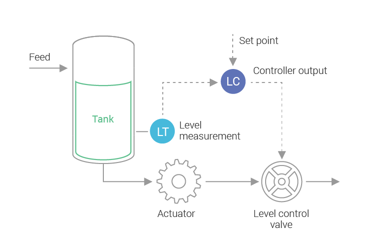
Let’s look at another example of a real-world closed-loop control system: we want the water in a water tank to be at or around a certain level, we will have a valve working as an actuator, and the difference between the current level and the desired level is the error. The controller will open or close the valve so that more or less water flows from the tank. How much the valve should open is determined by the transfer function of the controller. Figure 1 shows a simple diagram of this general idea.
![]()
Figure 1: An industrial controller, controlling the water level in a tank. The current level is measured and fed to a feedback-loop controller. Based on that an actuator will adjust the rate of water flow in the tank. Systems like this are commonly used in industrial plants. We can leverage that knowledge to control database processes as well.
The Pieces of the Puzzle: Schedulers and the Backlog Controller
Inside Scylla, the foundation of our control processes are the Schedulers embedded in the database. We discussed the earliest of them, the I/O Scheduler, extensively in a three-part article (part 1, part 2, and part 3). The Schedulers work as the actuators in a control system. By increasing the shares of a certain component we increase the rate at which that process is executed—akin to the valve in Figure 1 allowing more (or less) fluid to pass through. Scylla also embeds a CPU Scheduler, which plays a similar role for the amount of CPU used by each of the database’s internal processes.
To design our controller it’s important to start by reminding ourselves of the goal of compactions. Having a large amount of uncompacted data will lead to a read to both read amplification and space amplification. We have read amplification because each read operation will have to read from many SSTables, and space amplification because overlapping data will be duplicated many times. Our goal is to get rid of this amplification.
We can then define a measurement of how much work remains to be done to bring the system to a state of zero amplification. We call that the backlog. Whenever  new bytes are written into the system, we generate
  bytes of backlog into the future. Note that there isn’t a one-to-one relationship between
  and
and  , since we may have to rewrite the data many times to achieve a state of zero amplification. When the backlog is zero, everything is fully compacted and there is no read or write amplification.
We are still within our goal if we allow the system to accumulate backlog, as long as the backlog doesn’t grow out of bounds. After all, there isn’t a need to compact all work generated by incoming writes now. The amount of bandwidth used by all components will always add up to a fixed quantity—since the bandwidth of CPU and disk are fixed and constant for a particular system. If the compaction backlog accumulates, the controller will increase the bandwidth allocated to compactions, which will cause the bandwidth allocated to foreground writes to be reduced. At some point, a system in a steady state should reach equilibrium.
Different workloads have a different steady-state bandwidth. Our control law will settle on different backlog measures for them; a high-bandwidth workload will have a higher backlog than a low-bandwidth workload. This is a desirable property: higher backlog leaves more opportunity for overwrites (which reduce the overall amount of write amplification), while a low-bandwidth write workload will have a lower backlog, and therefore fewer SSTables and smaller read amplification.
With this in mind, we can write a transfer function that is proportional to the backlog.
Determining Compaction Backlog
Compaction of existing SSTables occurs in accordance with a specific compaction strategy, which selects which SSTables have to be compacted together, and which and how many should be produced. Each strategy will do different amounts of work for the same data. That means there isn’t a single backlog controller—each compaction strategy has to define its own. Scylla supports the Size Tiered Compaction Strategy (STCS), Leveled Compaction Strategy (LCS), Time Window Compaction Strategy (TWCS) and Date Tiered Compaction Strategy (DTCS).
In this article, we will examine the backlog controller used to control the default compaction strategy, the Size Tiered Compaction Strategy. STCS is described in detail in a previous post. As a quick recap, STCS will try to compact together SSTables of similar size. If at all possible, we try to wait until 4 SSTables of similar sizes are created and compact that. As we compact SSTables of similar sizes, we may create much larger SSTables that will belong to the next tier.
In order to design the backlog controller for STCS, we start with a few observations. The first is that when all SSTables are compacted into a single SSTable, the backlog is zero as there is no more work to do. As the backlog is a measure of work still to be done for this process, this follows from the definition of the backlog.
The second observation is that the larger the SSTables, the larger the backlog. This is also easy to see intuitively. Compacting 2 SSTables of 1MB each should be much easier on the system than compacting 2 SSTables of 1TB each.
A third and more interesting observation is that the backlog has to be proportional to the number of tiers that a particular SSTable still have to move through until it is fully compacted. If there is a single tier, we’ll have to compact the incoming data being currently written with all the SSTables in that tier. If there are two tiers, we’ll compact the first tier but then will have to compact every byte present in that tier – even the ones that were already sealed in former SSTables into another tier.
Figure 2 shows that in practice. As we write a new SSTable, we are creating a future backlog as that new SSTable will have to be compacted with the ones in its tier. But if there is a second tier, then there will be a second compaction eventually, and the backlog has to take that into account.
![]()
Figure 2: SSTables shown in blue are present in the system already when a new SSTable is being written. Because those existing SSTables live in two different Size Tiers, the new SSTable creates a future backlog roughly twice as big as if we had a single tier—since we will have to do two compactions instead of one.
Note that this is valid not only for the SSTable that is being written at the moment as a result of data being flushed from memory—it is also valid for SSTables being written as a result of other compactions moving data from earlier tiers. The backlog for the table resulting from a previous compaction will be proportional to the number of levels it still has to climb to the final tier.
It’s hard to know how many tiers we have. That depends on a lot of factors including the shape of the data. But because the tiers in STCS are determined by the SSTable sizes, we can estimate an upper bound for the number of tiers ahead of a particular SSTable based on a logarithmic relationship between the total size in the table for which the backlog is calculated and the size of a particular SSTable— since the tiers are of exponentially larger sizes.
Consider, for example, a constant insert workload with no updates that continually generates SSTables sized 1GB each. They get compacted into SSTables of size 4GB, which will then be compacted into SSTables of size 16GB, etc.
When the first two tiers are full, we will have four SSTables of size 1GB and four more SSTables of size 4GB. The total table size is 4 * 1 + 4 * 4 = 20GB and the table-to-SSTable ratios are 20/1 and 20/4 respectively. We will use the base 4 logarithm, since there are 4 SSTables being compacted together, to yield for the 4 small SSTables:
![\[ tier = log_4(20/1) = 2.1 \]]( "Rendered by QuickLaTeX.com")
and for the large ones
![\[ tier = log_4(20 / 4) = 1.1 \]]( "Rendered by QuickLaTeX.com")
So we know that the first SSTable, sized 1GB, belongs to the first tier while the SSTable sized 4GB belongs in the second.
Once that is understood, we can write the backlog of any existing SSTable that belongs to a particular table as:
![\[ B_i = S_i log_4( \frac{\sum _{i=0}^{N} S_i }{S_i}) \]]( "Rendered by QuickLaTeX.com")
where  is the backlog for SSTable
  ,
,  is the size of SSTable
  . The total backlog for a table is then
![\[ B = \sum_{i=0}^{N}{S_i log_4( \frac{\sum _{i=0}^{N} S_i }{S_i}) } \]]( "Rendered by QuickLaTeX.com")
To derive the formula above, we used SSTables that are already present in the system. But it is easy to see that it is valid for SSTables that are undergoing writes as well. All we need to do is to notice that  is, in fact, the partial size of the SSTable—the number of bytes written so far.
The backlog increases as new data is written. But how does it decrease? It decreases when bytes are read from existing SSTables by the compaction process. We will then adjust the formula above to read:
![\[ B = \sum_{i=0}^{N}{S_i log_4( \frac{\sum _{i=0}^{N} (S_i - C_i) }{(S_i - C_i)}) } \]]( "Rendered by QuickLaTeX.com")
where  is the number of bytes already read by compaction from sstable
  . It will be 0 in SSTables that are not undergoing compactions.
Note that when there is a single SSTable,  , and since
  , there is no backlog left—which agrees with our initial observations.
The Compaction Backlog Controller in Practice
To see this in practice, let’s take a look at how the system responds to an ingestion-only workload, where we are writing 1kB values into a fixed number of random keys so that the system eventually reaches steady state.
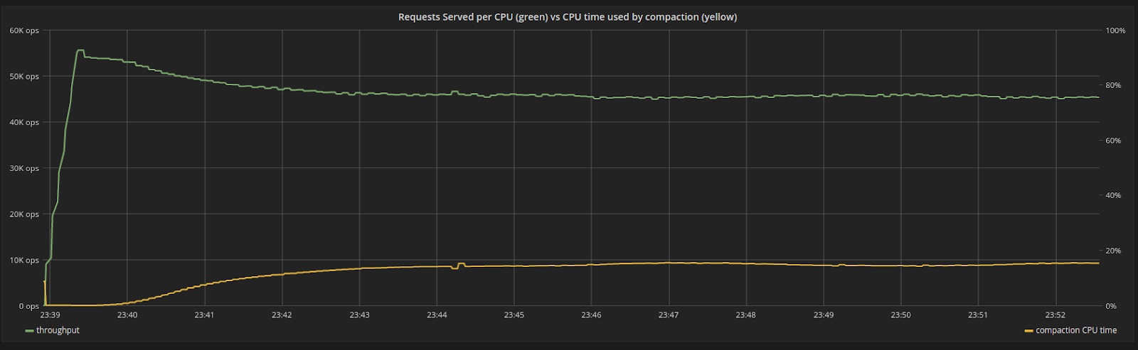
We will ingest data at maximum throughput, making sure that even before any compaction starts, the system is already using 100% of its resources (in this case, it is bottlenecked by the CPU), as shown in Figure 3. As compactions start, the internal compaction process uses very little CPU time in proportion to its shares. Over time, the CPU time used by compactions increases until it reaches steady state at around 15%. The proportion of time spent compacting is fixed, and the system doesn’t experience fluctuations.
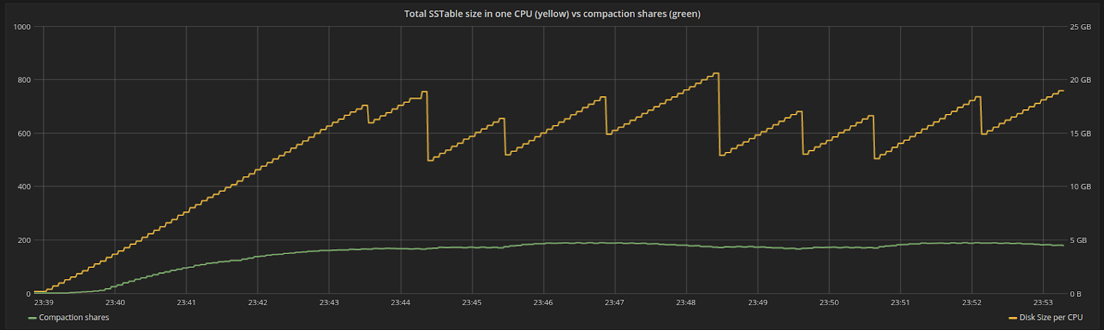
Figure 4 shows the progression of shares over time for the same period. Shares are proportional to the backlog. As new data is flushed and compacted, the total disk space fluctuates around a specific point. At steady state, the backlog sits at a constant place where we are compacting data at the same pace as new work is generated by the incoming writes.
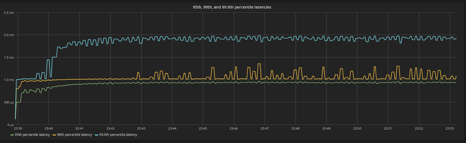
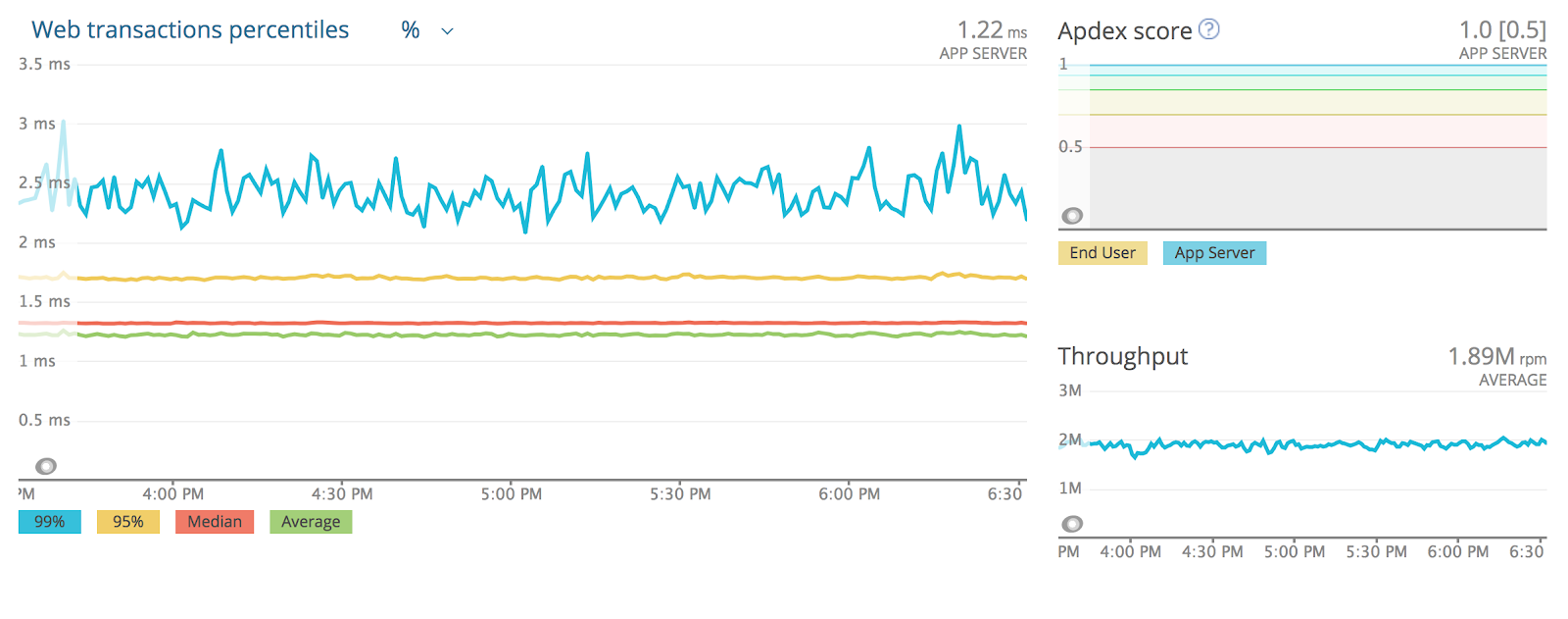
A very nice side effect of this is shown in Figure 5. Scylla CPU and I/O Schedulers enforce the amount of shares assigned to its internal processes, making sure that each internal process consumes resources in the exact proportion of their shares. Since the shares are constant in steady state, latencies, as seen by the server, are predictable and stable in every percentile.
![]()
Figure 3: Throughput of a CPU in the system (green), versus percentage of CPU time used by compactions (yellow). In the beginning, there are no compactions. As time progresses the system reaches steady state as the throughput steadily drops.
![]()
Figure 4: Disk space assigned to a particular CPU in the system (yellow) versus shares assigned to compaction (green). Shares are proportional to the backlog, which at some point will reach steady state
![]()
Figure 5: 95th, 99th, and 99.9th percentile latencies. Even under 100% resource utilization, latencies are still low and bounded.
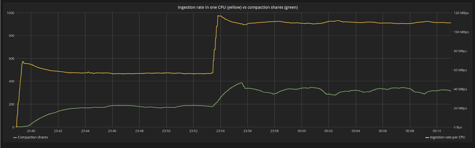
Once the system is in steady state for some time, we will suddenly increase the payload of each request, leading the system to ingest data faster. As the rate of data ingestion increases, the backlog should also increase. Compactions will now have to move more data around.
We can see the effects of that in Figure 6. With the new ingestion rate, the system is disturbed as the backlog grows faster than before. However, the compaction controller will automatically increase shares of the internal compaction process and the system will reach a new equilibrium.
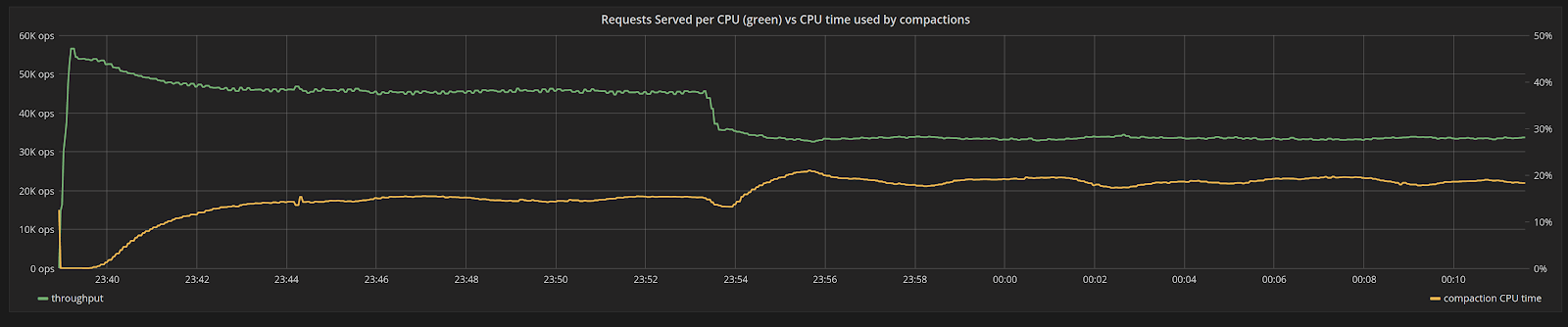
In Figure 7 we revisit what happens to the percentage of CPU time assigned to compactions now that the workload changes. As requests get more expensive the throughput in request/second naturally drops. But, aside from that, the larger payloads will lead to compaction backlog accumulating quicker. The percentage of CPU used by compactions increases until a new equilibrium is reached. The total drop in throughput is a combination of both of those effects.
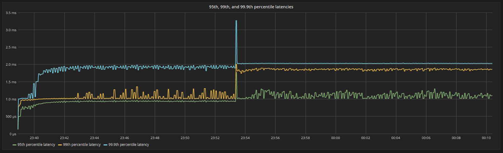
Having more shares, compactions are now using more of the system resources, disk bandwidth, and CPU. But the amount of shares is stable and doesn’t have wide fluctuations leading to a predictable outcome. This can be observed through the behavior of the latencies in Figure 8. The workload is still CPU-bound. There is now less CPU available for request processing, as more CPU is devoted to compactions. But since the change in shares is smooth, so is the change in latencies.
![]()
Figure 6: The ingestion rate (yellow line) suddenly increases from 55MB/s to 110MB/s, as the payload of each request increases in size. The system is disturbed from its steady state position but will find a new equilibrium for the backlog (green line).
![]()
Figure 7: Throughput of a CPU in the system (green), versus percentage of CPU time used by compactions (yellow) as the workload changes. As requests get more expensive the throughput in request/second naturally drops. Aside from that, the larger payloads will lead to compaction backlog accumulating quicker. The percentage of CPU used by compactions increases.
![]()
Figure 8: 95th, 99th and 99.9th percentile latencies after the payload is increased. Latencies are still bounded and move in a predictable way. This is a nice side effect of all internal processes in the system operating at steady rates.
Conclusions
At any given moment, a database like ScyllaDB has to juggle the admission of foreground requests with background processes like compactions, making sure that the incoming workload is not severely disrupted by compactions, nor that the compaction backlog is so big that reads are later penalized.
In this article, we showed that isolation among incoming writes and compactions can be achieved by the Schedulers, yet the database is still left with the task of determining the amount of shares of the resources incoming writes and compactions will use.
Scylla steers away from user-defined tunables in this task, as they shift the burden of operation to the user, complicating operations and being fragile against changing workloads. By borrowing from the strong theoretical background of industrial controllers, we can provide an Autonomous Database that adapts to changing workloads without operator intervention.
As a reminder, Scylla 2.2 is right around the corner and will ship with the Memtable Flush controller and the Compaction Controller for the Size Tiered Compaction Strategy. Controllers for all compaction strategies will soon follow.
Next Steps
- Learn more about Scylla from our product page.
- See what our users are saying about Scylla.
- Download Scylla. Check out our download page to run Scylla on AWS, install it locally in a Virtual Machine, or run it in Docker.
- Take Scylla for a Test drive. Our Test Drive lets you quickly spin-up a running cluster of Scylla so you can see for yourself how it performs.
The post Taming the Beast: How Scylla Leverages Control Theory to Keep Compactions Under Control appeared first on ScyllaDB.


 Choosing the Right NoSQL Datastore: Journeying From Apache Cassandra to Scylla


 new bytes are written into the system, we generate
  bytes of backlog into the future. Note that there isn’t a one-to-one relationship between
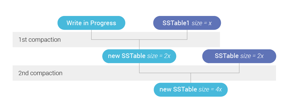
![\[ tier = log_4(20/1) = 2.1 \]](http://www.scylladb.com/wp-content/ql-cache/quicklatex.com-a3334465b2fd8dba4e245d37c01b8810_l3.png "Rendered by QuickLaTeX.com")
![\[ tier = log_4(20 / 4) = 1.1 \]](http://www.scylladb.com/wp-content/ql-cache/quicklatex.com-6d3bd233f2e0374cedc322257584472a_l3.png "Rendered by QuickLaTeX.com")
![\[ B_i = S_i log_4( \frac{\sum _{i=0}^{N} S_i }{S_i}) \]](http://www.scylladb.com/wp-content/ql-cache/quicklatex.com-963cbdb3989789b7398180b0c9523b43_l3.png "Rendered by QuickLaTeX.com")
 is the backlog for SSTable
  ,
,  is the size of SSTable
  . The total backlog for a table is then
![\[ B = \sum_{i=0}^{N}{S_i log_4( \frac{\sum _{i=0}^{N} S_i }{S_i}) } \]](http://www.scylladb.com/wp-content/ql-cache/quicklatex.com-1522f9c4dc1cd56dd6b63e88ba369798_l3.png "Rendered by QuickLaTeX.com")
 is, in fact, the partial size of the SSTable—the number of bytes written so far.
![\[ B = \sum_{i=0}^{N}{S_i log_4( \frac{\sum _{i=0}^{N} (S_i - C_i) }{(S_i - C_i)}) } \]](http://www.scylladb.com/wp-content/ql-cache/quicklatex.com-e5b6072f901cb4eabdb1240f3e0b7e0f_l3.png "Rendered by QuickLaTeX.com")
 is the number of bytes already read by compaction from sstable
  , and since
  , there is no backlog left—which agrees with our initial observations.